


Introduction
As computational tools become increasingly accessible and user-friendly, even for relatively inexperienced engineers, the need for critical evaluation of computational analyses has grown correspondingly. In the field of structural steel design, the finite element analysis (FEA) of structural connections represents the next rapidly advancing step. However, the reliability of such analyses can only be established through a systematic process of verification and validation (V&V). Without rigorous V&V, finite element results lack credibility and cannot serve as a basis for engineering decision-making.
The present article revisits selected chapters from Component-Based Finite Element Design of Steel Connections by František Wald et al., recalculated using the most recent release of IDEA StatiCa software. In addition, several chapters have been expanded through supplementary examples, thereby enhancing the robustness and accuracy of the verification process. This contribution aims to strengthen the methodological foundations of connection design and provide a more reliable reference for both academic research and engineering practice.

Theoretical background
You can find the description of the CBFEM method in two separate Theoretical background online documents:
IDEA StatiCa Connection – Structural design of steel connections - general introduction to the CBFEM method and analysis model inside the Connection app.
Check of steel connection components (EN) - description of the implementation of Eurocode (EN) regarding the required checks.
IDEA StatiCa Member – Member stability - general introduction to the stability, buckling, and geometrically nonlinear analysis with imperfections (GMNIA) calculation method inside the Member app.
Welded connections
Fillet weld in lap joint
Description
The objective of this chapter is the verification of the component-based finite element method (CBFEM) of a fillet weld in a lap joint with the component method (CM). Two plates are connected in three configurations, namely with a transverse weld, with a longitudinal weld, and a combination of transverse and longitudinal welds. The length and throat thickness of the weld are the varying parameters in the study. The study also covers long welds whose resistance is reduced due to stress concentration. The joint is loaded by a normal force.
Analytical model
The fillet weld is the only component examined in the study. The welds are designed to be the weakest component in the joint. The weld is designed according to EN 1993-1-8:2005. The design resistance of the fillet weld is determined using the Directional method given in Cl. 4.5.3.2 in EN 1993-1-8:2005. The available calculation methods for checking the strength of fillet welds are based upon the simplifying assumption that stresses are uniformly distributed within a throat section of a fillet weld, leading to the normal stresses and shear stresses shown in Fig. 4.1.1, as follows:
- σ⊥ is the normal stress perpendicular to the throat section;
- σ∥ is the normal stress parallel to the axis of the weld in its cross-section;
- τ⊥ is the shear stress (in the plane of the throat section) perpendicular to the axis of the weld;
- τ∥ is the shear stress (in the plane of the throat section) parallel to the axis of the weld.
The normal stress σ∥ parallel to the axis is not considered when verifying the design resistance of a weld.

The design resistance of the fillet weld will be sufficient if the following are both satisfied:
In lap joints longer than , the reduction factor is given by:
but
Numerical model
The weld component in CBFEM is described in General theoretical background and EN theoretical background. Nonlinear elastic-plastic material is used for welds in this study. The limiting plastic strain is reached in the longer part of the weld, and stress peaks are redistributed.
Verification of resistance
An overview of the considered examples and the material properties is provided in Tab. 4.1.1. The weld configurations are T for transverse, P for parallel weld, and TP for a combination of both; see the geometry in Fig. 4.1.2. The steel grade was S235 (fy = 235 MPa, fu = 360 MPa, E = 210 GPa, βw = 0,8). Partial safety factors were γM0 = 1.0, γM2 = 1.25. The geometry of the model is shown in Fig. 4.1.2. The plates have a thickness of 20 mm. The connection is symmetrical, and the plate is pulled out of the welded splice connection. The length and width of the plates are adjusted according to the length of the parallel and transverse weld. The weld resistance is always the governing failure mode. The weld throat thickness is 3 mm. The lengths of the transverse and parallel welds vary in this parametric study.

Design weld resistance calculated by CBFEM is compared with the results of CM. The results are presented in Tab. 4.1.1 – 4.1.3 and Fig. 4.1.3 – 4.1.5.

Transverse welds resistance calculation
Where:
- weld throat thickness
- the normal force acting on the beam
- total transverse weld length
- correlation factor taken from EN 1993-1-8 Table 4.1
- nominal ultimate tensile strength of the weaker part joined
- partial safety factor for welds
Parallel weld resistance calculation
Where:
- weld throat thickness
- shear force acting on beam
- total parallel welds length
- correlation factor taken from EN 1993-1-8 Table 4.1
- long weld reduction factor, EN 1993-1-8 Equation 4.9
- nominal ultimate tensile strength of the weaker part joined
- partial safety factor for welds
Transverse and parallel calculation
The resistance calculated by hand for a transverse and parallel weld combination is simply the sum of the transverse and parallel resistances derived from the equations above.
Results Presentation


The resistance of parallel welds, transverse welds, and multi-oriented weld groups is nearly identical according to CM and CBFEM. The biggest difference in this study is 6% in load resistance.
The CBFEM results of parallel welds are slightly conservative but start to diverge for long welds. The reduction of resistance due to long welds is not captured by CBFEM, but it is not expected that welds longer than 200×throat thickness could appear in any connection, and up to this length, the results are still very close.
For transverse welds, CBFEM provides very consistent results with 2–4% higher resistance.
Benchmark example
Inputs
Member 1 – Iw60x500
• Welded from plates with thickness t = 20 mm
• Width b = 500 mm
• Web is removed by Opening manufacturing operation
• Steel S235
Member 2 – Plate 20x1000
• Thickness t = 20 mm
• Width b = 1000 mm
• Steel S235
• Offset ex = –90 mm
Transverse fillet weld at both sides of Member 2
• Throat thickness a = 3 mm
• Weld length Lt = 100 mm
Parallel fillet weld at both sides of Member 2
• Throat thickness a = 3 mm
• Weld length Lp = 100 mm
Output
• Design resistance in tension FRd = 387 kN (It should be noted that the resistance was calculated using the "Stop at limit strain" function. Consequently, the actual CBFEM resistance may be marginally higher.)
Fillet weld in angle plate joint
Description
In this chapter, the model of the fillet weld in angle plate joint calculated by component-based finite element method (CBFEM) is verified on component method (CM). An angle is welded to a plate and loaded by normal force. The angle size and the length of the weld are studied in a sensitivity study.
Analytical model
The fillet weld is the only component examined in the study. The welds are designed according to Chapter 4 in EN 1993-1-8:2005 to be the weakest component in the joint. The design resistance of the fillet weld is described in Section 4.1. Overview of considered examples and material is given in Tab. 4.2.1. The geometry of the joints with dimensions is shown in Fig. 4.2.1.
Component method calculation
This hand calculation neglects the additional moment of the weld, which is developed due to force redistribution to the L cross-section parts acc. to EN 1993-1-8 (4.13).
Total resistance calculated as sum of top and bottom weld resistances
Where:
- weld throat thickness
- shear force acting on beam
- parallel welds length
- correlation factor taken from EN 1993-1-8 Table 4.1
- long weld reduction factor, EN 1993-1-8 Equation 4.9
- nominal ultimate tensile strength of the weaker part joined
- partial safety factor for welds


Numerical model
The weld component in CBFEM is described in General theoretical background and EN theoretical background. The weld model has an elastic-plastic material diagram, and stress peaks are redistributed along the weld length.
Verification of resistance
The weld design resistances calculated by CBFEM are compared with the results of CM; see Tab. 4.2.2. Two parameters are studied: the length of the weld and the angle section. Fig 4.2.2 shows the sensitivity study of bottom weld length. The length of the top weld a in the study is La=100mm.


Results of CBFEM and CM are compared, and the sensitivity study is presented. The influence of weld length on the design resistance of a welded angle joint is shown in Fig. 4.2.2. The study shows good agreement for all weld configurations. To illustrate the accuracy of the CBFEM model, the results of the study are summarized in a diagram comparing design resistances by CBFEM and CM; see Fig. 4.2.3. The results show that all the predictions of CBFEM are safe-sided compared to the CM, where eccentricity is neglected.


Benchmark example
Inputs
Angle
- Cross-section 2×L80×10
- Distance between angles 16 mm
Plate
- Thickness tp = 16 mm
- Width bp = 240 mm
Weld, parallel fillet welds, see Fig. 4.2.4
- Throat thickness aw = 3 mm
- Top weld length Lw,top = 100 mm
- Bottom weld length Lw,bottom = 50 mm
Outputs
- Design resistance in tension FRd = 170 kN (It should be noted that the resistance was calculated using the "Stop at limit strain" function. Consequently, the actual CBFEM resistance may be marginally higher.)

Fillet weld in fin plate joint
Description
In this chapter, component-based finite element method (CBFEM) of a fillet weld in a fin plate joint is verified with component method (CM). A fin plate is welded to open section column HEB. The height of the fin plate is changed from 150 to 300 mm. The plate/weld is loaded by normal and shear force and bending moment.
Analytical model
The fillet weld is the only component examined in the study. The welds are designed to be the weakest component in the joint according to Chapter 4 in EN 1993-1-8:2005. The design resistance of the fillet weld is described in Section 4.1. Overview of considered examples and material is given in Tab. 4.3.1. Three load cases are considered: normal force N, shear force V, and bending moment M. Geometry of the joint with dimensions is shown in Fig. 4.3.1.
Weld normal resistance calculation
Where:
- weld throat thickness
- the normal force acting on the beam
- total weld length
- correlation factor taken from EN 1993-1-8 Table 4.1
- nominal ultimate tensile strength of the weaker part joined
- partial safety factor for welds
Weld bending resistance calculation
Where:
- weld throat thickness
- weld plastic section modulus
- bending moment acting on the beam
- total weld length
- correlation factor taken from EN 1993-1-8 Table 4.1
- nominal ultimate tensile strength of the weaker part joined
- partial safety factor for welds
Weld shear resistance calculation
Where:
- weld throat thickness
- shear force acting on beam
- total weld length
- correlation factor taken from EN 1993-1-8 Table 4.1
- nominal ultimate tensile strength of the weaker part joined
- partial safety factor for welds


Numerical model
The weld component in CBFEM is described in General theoretical background and EN theoretical background. The weld model has an elastic-plastic material diagram, and stress peaks are redistributed along the weld length.
Verification of resistance
Design resistance calculated by CBFEM is compared with the results of CM. The comparison is presented in Tab. 4.3.2. The study is performed for one parameter: length of the weld, i.e. height of the fin plate, and three load cases: normal and shear force and bending moment. The shear force is applied in a weld plane to neglect the effect of an additional bending. The bending moment is applied at the end of the fin plate. The influence of the weld length on the design resistance of the fin plate joints loaded by the normal and shear force are shown in Fig. 4.3.2. The relation between the weld length and the bending moment resistance of the joint is shown in Fig. 4.3.3.

The results of CBFEM and CM are compared, and the sensitivity study is presented. The influence of weld length on the design resistance in a fin plate joint loaded by normal force is shown in Fig. 4.3.2, by shear force in Fig. 4.3.3, and by bending moment in Fig. 4.3.4. The study shows good agreement for all applied load cases.


To illustrate the accuracy of the CBFEM model, the results of the parametric studies are summarized in a diagram comparing the design resistances of CBFEM and CM; see Fig. 4.3.5. The results show that the difference between the two calculation methods is in all cases less than 10 %.


Benchmark example
Inputs
Column
- Steel S235
- HEB 400
Fin plate
- Thickness tp = 15 mm
- Height hp = 175 mm
Weld, double fillet weld, see Fig. 4.3.6
- Throat thickness aw = 3 mm
Outputs
- Design resistance in pure bending MRd = 11.4 kNm

Fillet weld in beam to column joint
Description
The object of this chapter is verification of component based finite element method (CBFEM) for a fillet weld in a stiffened beam-to-column joint with component method (CM). An open section beam IPE is connected to open section column HEB400. The stiffeners are inside column opposite to beam flanges. The beam section is the changing parameter. Three load cases are considered, i.e. the beam is loaded in tension, shear and bending.
Analytical model
The fillet weld is the only component examined in the study. The welds are designed according to Chapter 4 in EN 1993-1-8:2005 to be the weakest component in the joint. The design resistance of the fillet weld is described in Section 4.1. Overview of the considered examples and the material are given in the Tab. 4.4.1. A geometry of the joint with dimensions is shown in Fig. 4.4.1.
Tab. 4.4.1 Examples overview

Hand Calculation of normal force N
Where:
- weld throat thickness
- normal force acting on beam
- total welds length
- correlation factor taken from EN 1993-1-8 Table 4.1
- nominal ultimate tensile strength of the weaker part joined
- partial safety factor for welds
Hand Calculation of shear force V
The manual calculation presented in this chapter is predicated on certain assumptions. The shear force is transmitted exclusively by the weld at the web. The bending moment resulting from the eccentricity of the force acting on the welds can be attributed to the flange welds. The weld section modulus of flange welds is determined not by the distance measured from the centre of gravity of the welds, but from the edges of the flange to the beam centre of gravity, as calculated in practice.
The following equations demonstrate the derivation of the weld load-bearing capacity for shear force and bending moment according to the CM. The equivalent stress is specified in EN 1993-1-8, Equation (4.1). For the calculation of bending moment resistance, the plastic section modulus was assumed.
Where:
- force eccentricity relative to the beam welds
- weld throat thickness
- shear force acting on beam
- welds section modulus
- top flange edge weld area
- bottom flange edge weld area
- top flange edge weld lever arm
- bottom flange edge weld lever arm
- plastic flange section modulus
- total web welds length
- correlation factor taken from EN 1993-1-8 Table 4.1
- nominal ultimate tensile strength of the weaker part joined
- partial safety factor for welds
- IPE beam height
- IPE beam width
- IPE beam web thickness
- IPE beam flange thickness
Hand Calculation of bending moment M
In the calculation of bending moment without any interaction with shear force, the plastic section modulus of the whole weld section (both around flanges and around web) was assumed.
Where:
- weld throat thickness
- weld plastic section module
- the bending moment acting on the beam
- correlation factor taken from EN 1993-1-8 Table 4.1
- nominal ultimate tensile strength of the weaker part joined
- partial safety factor for welds
Numerical model
The weld component in CBFEM is described in General theoretical background and EN theoretical background.
Nonlinear elastic-plastic material is used for welds in this study. The limit plastic strain is reached in longer part of the weld and stress peaks are redistributed.

Verification of resistance
Design resistance calculated by CBFEM Idea RS software is compared with the results of CM. The weld’s design resistances are compared, see Tab. 4.4.2. The study is performed for one parameter beam section and three load cases: normal force NEd, shear force VEd, and bending moment MEd.
Tab. 4.4.2 Comparison of CBFEM and CM

Results of CBFEM and CM are compared and a sensitivity study is presented. The influence of beam cross-section on the design resistance a welded beam-to-column joint loaded in tension is shown in Fig. 4.4.2, in shear in Fig. 4.4.3 and in bending in Fig. 4.4.4. The study shows good agreement for all applied load cases.


To illustrate the accuracy of the CBFEM model, results of the sensitivity study is summarized in a diagram comparing CBFEM’s and CM’s design resistances, see Fig. 4.4.5. The results show that the difference of the two calculation methods is in all cases less than 10%.


Benchmark example
Inputs
Column
- Steel S235
- HEB 400
Beam
- Steel S235
- IPE 160
- Force eccentricity to weld x = 400 mm, see Fig. 4.4.6
Weld
- Throat thickness aw = 3 mm
Outputs:
- Design resistance in shear VRd = 105 kN

Connection to unstiffened flanges
Description
In this chapter, component-based finite element method (CBFEM) of a fillet weld connecting a plate to an unstiffened column is verified on component method (CM). The steel plate is connected to the open and box section columns and loaded in tension.
Analytical model
The fillet weld is the only component examined in the study. The welds are designed according to Chapter 4 in EN 1993-1-8:2005 to be the weakest component in the joint. The design resistance of the fillet weld is described in Section 4.1. The force applied perpendicular to a flexible plate, which is welded to an unstiffened section, is limited. The stresses are concentrated in an effective width while the weld resistance around the unstiffened parts is neglected, as shown in Fig. 4.5.1. For an unstiffened I or H section the effective width is obtained according to:
The dimension s is for a rolled section and for a welded section . For a box or channel section, the effective width should be obtained from:
Where:
- weld throat thickness
- normal force acting on beam
- total effective welds length
- correlation factor taken from EN 1993-1-8 Table 4.1
- nominal ultimate tensile strength of the weaker part joined
- partial safety factor for welds

Numerical model
The weld component in CBFEM is described in General theoretical background and EN theoretical background. The plastic branch is reached in a part of the weld, and stress peaks are redistributed along the weld length.
Verification of resistance
Design resistance calculated by CBFEM is compared with the results of CM. The weld design resistance is compared only. Overview of considered examples and material is given in Tab. 4.5.1. Geometry of joints with dimensions is shown in Fig. 4.5.2.


The results are presented in Tab. 4.5.2. The study is performed for two parameters: flange width of the HEB section and web thickness of the box section. The flexible plate is loaded in tension. The influence of the flange width of HEB section on design resistance of a joint is shown in Fig. 4.5.3. The relation between the web thickness of box section on design resistance of a joint is shown in Fig. 4.5.4.

Results of CBFEM and CM are compared in a sensitivity study. The influence of the flange width of HEB section on design resistance of a joint is studied in Fig. 4.5.3. The influence of the web thickness of box section on design resistance of a joint is presented in Fig. 4.5.4. The parametric studies show very good agreement of the results for all weld configurations.


The results of the sensitivity study are summarized in a diagram comparing design resistances of CBFEM and CM; see Fig. 4.5.5 illustrating the accuracy of the CBFEM model.


The influence of the plate thickness on the design resistance of the weld is shown in Fig. 4.5.6. The column cross-section is HEB 180 with a flange thickness of 14 mm. A weld connecting a plate thicker than the column flange has the same resistance for CM and CBFEM. On the other hand, the weld connecting the plate to column flange of the same or smaller thickness has in numerical models design resistance smaller by 20%. The plate thickness is not taken into account in numerical models with shell elements, which causes the difference.

Benchmark example
Inputs
Column
• Steel S235
• RHS 200/200/5
Flexible plate
• Steel S235
• Thickness tp = 17 mm
• Width bp = 190 mm
Weld, double fillet welds see Fig. 4.5.7
• Throat thickness aw = 5 mm
Outputs
• Design resistance in tension NRd = 68 kN

Bolted connections
Bolted connection - T-stub in tension
Description
The objective of this chapter is verification of component-based finite element method (CBFEM) of T-stubs connected with two bolts loaded in tension with component method (CM) and research FEM model (RM) created in Midas FEA software; see (Gödrich et al. 2019).
Analytical model
Welded T-stub and bolt in tension are components examined in the study. Both components are designed according to EN 1993-1-8:2005. The welds are designed not to be the weakest component. Effective lengths for circular and noncircular failures are considered according to EN 1993-1-8:2005 cl. 6.2.6. Only tension loads are considered. Three modes of collapse according to EN 1993-1-8:2005 cl. 6.2.4.1 are considered: 1. mode with full yielding of the flange, 2. mode with two yield lines by web and rupture of the bolts, and 3. mode for rupture of the bolts; see Fig. 5.1.1. Bolts are designed according to cl. 3.6.1 in EN 1993-1-8:2005. Design resistance considers punching shear resistance and rupture of the bolt.

Design numerical model
T-stub is modeled by 4-nodes shell elements as described in Chapter 3 and summarised further. Every node has 6 degrees of freedom. Deformations of the element consist of membrane and flexural contributions. Nonlinear elastic-plastic material status is investigated in each layer of integration point. Assessment is based on the maximum strain given according to EN 1993‑1‑5:2006 by value of 5 %. Bolts are divided into three sub-components. The first is the bolt shank, which is modeled as a nonlinear spring and caries tension only. The second sub-component transmits tensile force into the flanges. The third sub-component solves shear transmission.
Research numerical model
In cases where the CBFEM gives higher resistance, initial stiffness, or deformation capacity, research FEM model (RM) from brick elements validated on experiments (Gödrich et al. 2013) is used to verify the CBFEM model. RM is created in Midas FEA software of hexahedral and octahedral solid elements, see Fig. 5.1.2 Mesh sensitivity study was provided to reach proper results in adequate time. Numerical model of the bolts is based on the model by (Wu et al. 2012). The nominal diameter is considered in the shank, and the effective core diameter is considered in the threaded part. Washers are coupled with the head and nut. Deformation caused by stripping of the threads in thread–nut contact area is modeled using interface elements. Interface elements are unable to transfer tensile stresses. Contact elements allowing the transmission of pressure and friction are used between washers and flanges of the T-stub. One-quarter of the sample was modeled using the symmetry.


Range of validity
CBFEM was verified for the selected typical T-stub geometries. The minimal thickness of the flange is 8 mm. Maximal distance of the bolts to bolt diameter is limited by p/db ≤ 20. The distance of the bolt line to the web is limited to m/db ≤ 5. Overview of the considered samples with steel plates of S235: fy = 235 MPa, fu = 360 MPa, E = Ebolt = 210 GPa is shown in the Tab. 5.1.1 and in Fig. 5.1.3.
Tab. 5.1.1 Overview of the considered samples of T stubs

Global behavior
Comparison of the global behavior of the T-stub described by force–deformation diagrams for all design procedures was prepared. Attention was focused on the main characteristics: initial stiffness, design resistance, and deformation capacity. Sample tf20 was chosen to present as a reference; see Fig. 5.1.4 and Tab. 5.1.2. CM generally gives higher initial stiffness compared to CBFEM and RM. In all cases, RM gives the highest design resistance, as shown in chapter 6. Deformation capacity is also compared. Deformation capacity of T-stub was calculated according to (Beg et al. 2004). RM does not consider cracking of the material, so the prediction of deformation capacity is limited.

Tab. 5.1.2 Global behavior overview

Verification of resistance
Design resistances calculated by CBFEM were compared with the results of CM and RM in the next step. The comparison was focused on the deformation capacity and determination of the collapse mode too. All results are ordered in Tab. 5.1.3. The study was performed for five parameters: thickness of the flange, bolt size, bolt material, bolt space, and T-stub width.
Tab. 5.1.3 Global behavior overview


The sensitivity study of thickness of the flange shows higher resistance according to CBFEM compared to CM for samples with flange thicknesses up to 20 mm. RM gives even higher resistance for these samples; see Fig. 5.1.5. Higher resistance of both numerical models is explained by neglecting membrane effect in CM. In case of the bolt diameter and bolt material (see Fig. 5.1.6 and Fig. 5.1.7, respectively), the results of CBFEM correspond to these of CM. Due to a good agreement of both methods, the results of RM are not required.


In the case of the bolt distances, the results of CBFEM and CM show generally good agreement; see Fig. 5.1.8. With an increase in bolt spacing, CBFEM gives slightly higher resistance compared to CM. For that reason, the results of RM are also shown. RM gives the highest resistance in all cases.

In the study of T-stub width, CBFEM shows higher resistance compared to CM with an increase in width. Results of RM were prepared, which again provide the highest resistance in all cases; see Fig. 5.1.9.

To show the prediction of the CBFEM model, the results of the studies were summarized in graph comparing resistances by CBFEM and CM; see Fig. 5.1.10. The results show that the difference between the two calculation methods is mostly up to 10 %. In cases with CBFEM/CM > 1,1, accuracy of CBFEM was verified by the results of RM, which gives the highest resistance in all selected cases.


Benchmark example
Inputs
T-stub, see Fig. 5.1.11
- Steel S235
- Flange thickness tf = 20 mm
- Web thickness tw = 20 mm
- Flange width bf = 300 mm
- Length b = 100 mm
- Double fillet weld aw = 10 mm
Bolts
- 2 × M24 8.8
- Distance of the bolts w = 165 mm
Code setup – Model and mesh
- Number of elements on biggest member or flange 16
Outputs
- Design resistance in tension FT,Rd = 164 kN
- Collapse mode – full yielding of the flange with maximal strain 5 %
- Utilization of the bolts 86,4 %
- Utilization of the welds 45,7 %

References
EN 1993-1-5, Eurocode 3, Design of steel structures – Part 1-5: Plated Structural Elements, CEN, Brussels, 2005.
EN 1993-1-8, Eurocode 3, Design of steel structures – Part 1-8: Design of joints, CEN, Brussels, 2005.
Beg D., Zupančič E., Vayas I. On the rotation capacity of moment connections, Journal of Constructional Steel Research, 60 (3–5), 2004, 601–620.
Gödrich L., Wald F., Sokol Z. To Advanced modelling of end plate joints, Connection and Joints in Steel and Composite Structures, Rzeszow, 2013.
Gödrich L., Wald F., Kabeláč J., Kuříková M. Design finite element model of a bolted T-stub connection component, Journal of Constructional Steel Research. 2019, (157), 198-206.
Wu Z., Zhang S., Jiang S. Simulation of tensile bolts in finite element modelling of semi-rigid beam-to-column connections, International Journal of Steel Structures 12 (3), 2012, 339-350.
Bolted connection - Splices in shear
Description
This study is focused on the verification of component-based finite element method (CBFEM) for the resistance of the symmetrical double splice bolted connection to an analytical model (AM).
Analytical model
The bolt resistance in shear and the plate resistance in bearing are designed according to Tab. 3.4 in chapter 3.6.1 in EN 1993-1-8:2005. For long connection, reduction factor according to cl. 3.8 is considered. Design resistance of connected members with reductions for fastener holes is taken into account according to cl 3.10.

Verification of resistance
Design resistances calculated by CBFEM were compared with results of analytical model (AM). Results are summarised in Tab. 5.2.1. The parameters are bolt material, splice thickness, bolt diameter, and bolt distances, see Figs. 5.2.1 to 5.2.4.


Tab. 5.2.1 Sensitivity study of resistance
Joint description: splice 150/10mm, bolts 2×M20 in distances p =70, e1=50, plates 2×150/6mm, steel S235

Joint description: splice height 200mm, bolts 3×M16 8,8 in distances p = 55mm e1 = 40mm, plates 2×200/t mm, steel S235

Joint description: splice 120/10mm, bolts 2×MX 8,8, plates 2×120/10 mm, steel S235

Joint description: Splice 200/6 mm, bolts 3×M16 8,8, plates 2×200/6mm, steel S235


The results of sensitivity studies are summarized in the graph in Fig. 5.2.5. The results show that the differences between the two calculation methods are below 5 %. The analytical model gives generally higher resistance.


Benchmark example
Inputs
Connected member
- Steel S235
- Splice 200/10 mm
Connectors
Bolts
- 3 × M16 8.8
- Distances e1 = 40 mm, p = 55 mm
2 x splice
- Steel S235
- Plate 380×200×10
Outputs
- Design resistance FRd = 258 kN
- Critical is bearing of the connected splice

End plate minor axis connection
Description
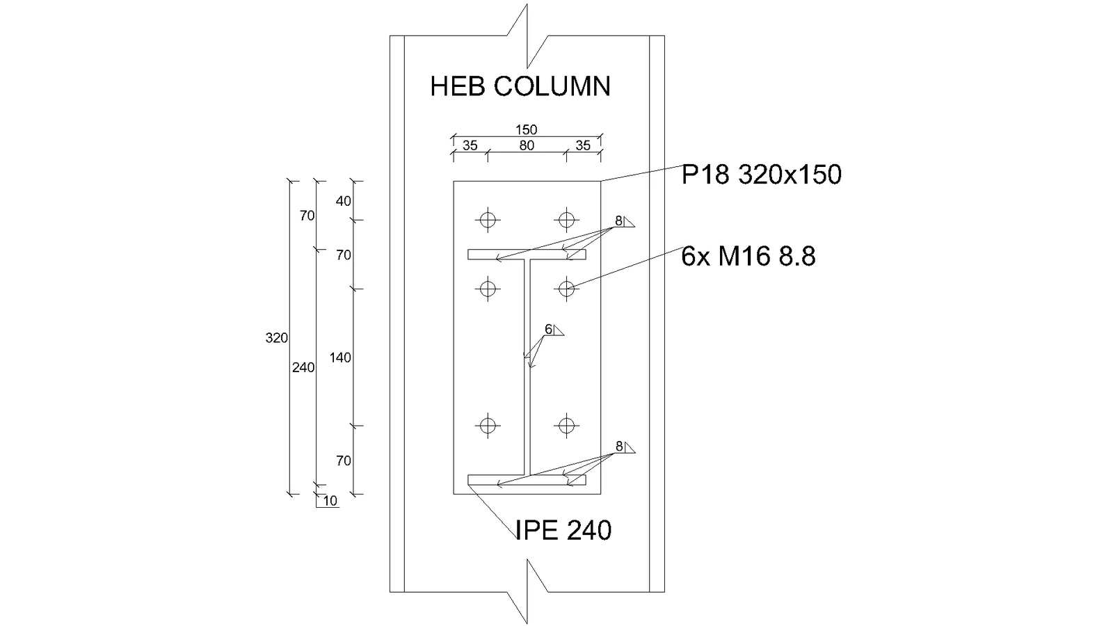
Component-based finite element method (CBFEM) model of the beam to column joint is verified on Component method (CM). The extended end plate with three bolt rows is connected to column web and loaded by bending moment; see Fig. 5.3.1.
Analytical model
Three components, which are guiding the behavior, are the end plate in bending, the beam flange in tension and in compression, and the column web in bending. The end plate and the beam flange in tension and in compression are designed according to EN 1993-1-8:2005. The behavior of the column web in bending is predicted according to (Steenhuis et al. 1998). The results of experiments of the beam to column minor axis joints, e.g. (Lima et al. 2009), show good prediction of this type of joint loaded in-plane of a connected beam.
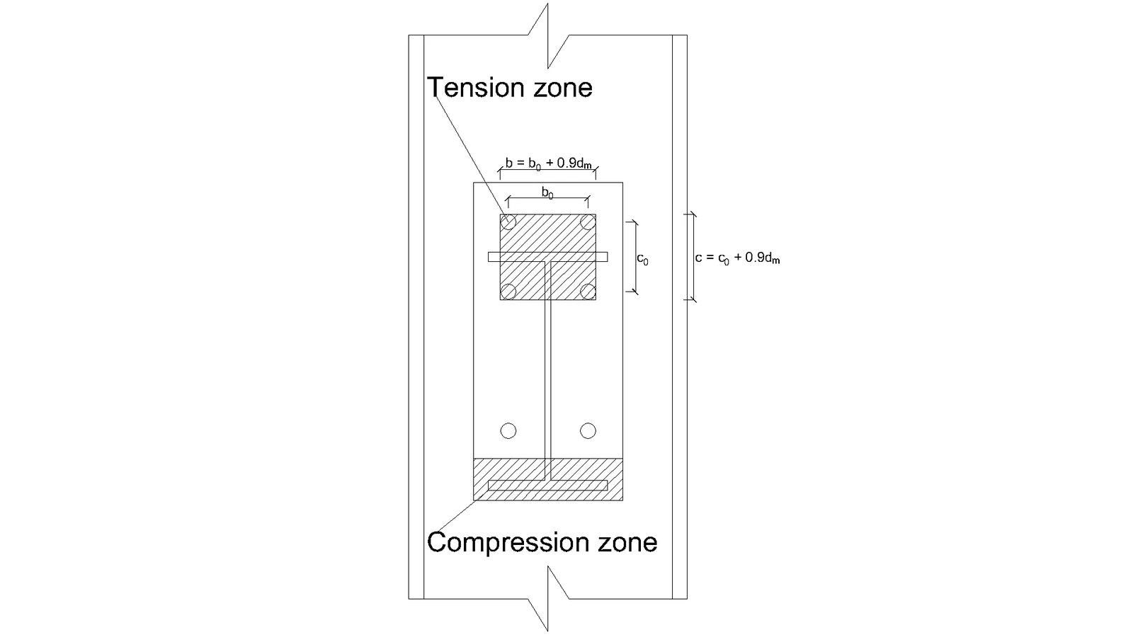
Where:
- is the thickness of the column web
- is the yield strength of the column web
- is the partial safety factor of steel
- is the partial safety factor of steel
- number bolt rows in tension
- bolt head diagonal diameter
- horizontal distance between bolts
- vertical distance between bolts
- lever arm of the joint
- is the resistance to punching shear
- is the resistance to combined punching, shear and bending
Numerical model
Assessment is based on the maximum strain given according to EN 1993-1-5:2006 by the value of 5 %. Detailed information about CBFEM model is summarized in Chapter 3.
Verification of resistance
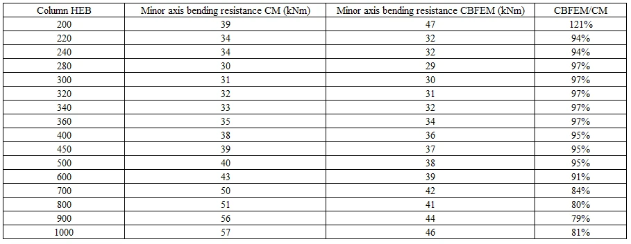
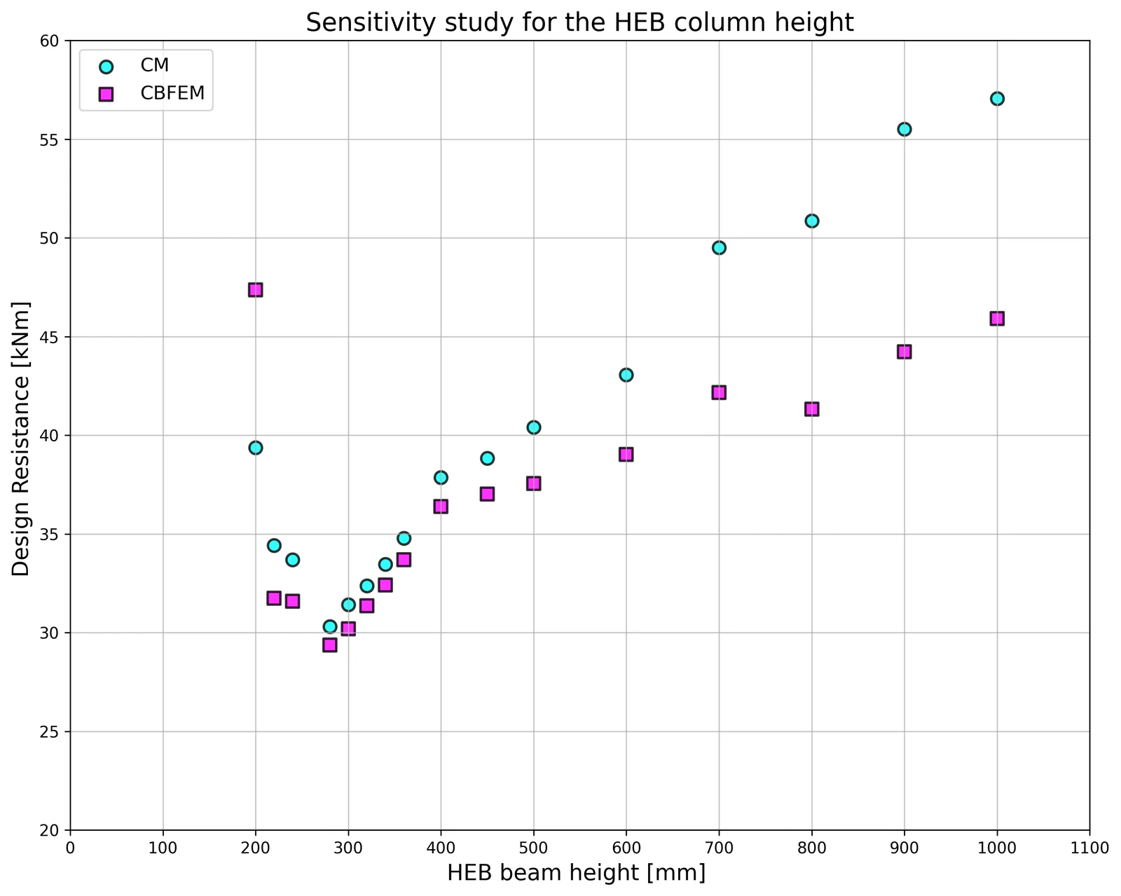
The sensitivity study of the joint resistance was prepared for column cross-sections. Joint geometry is shown in Fig. 5.3.1. In Tab. 5.3.1 and in Fig. 5.3.3, the results of calculations in case of enlarging end plate P18 relatively with the column section are summarized.
Tab. 5.3.1 Results of prediction of the of end plate minor axis connection for different rafters
Global behavior
Global behavior is presented on force-deformation curve. Beam IPE 240 is connected to column HEB 300 with six bolts M16 8.8. End plate geometry is shown in Fig. 5.3.1 and in Tab. 5.3.1. Comparison of both methods results is presented in Fig. 5.3.4 and in Tab.5.3.2. Both methods predict similar design resistance. CBFEM generally gives lower initial stiffness compared to CM.
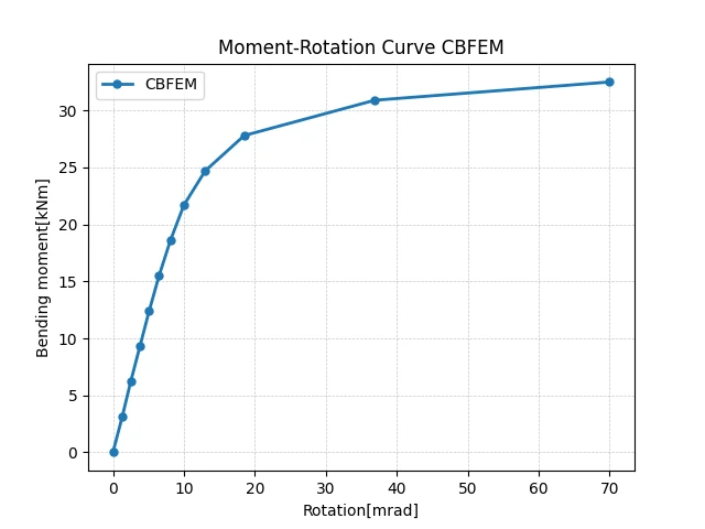
Tab. 5.3.2 Main characteristics for global behavior
| CM | CBFEM | CM/CBFEM | ||
| Initial stiffness | [kNm/rad] | 16130 | 2232 | 7.23 |
| Design resistance | [kNm] | 31 | 30 | 1,03 |
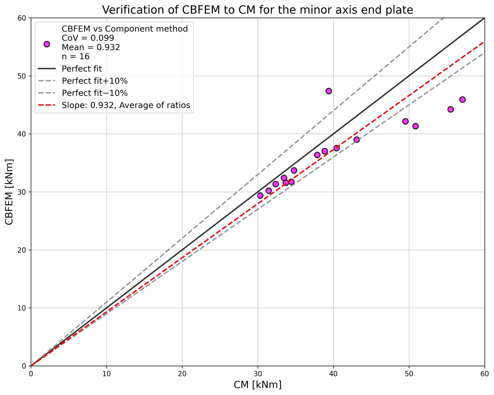
The results of studies are summarized in the graph comparing resistances by CBFEM and component method; see Fig. 5.3.5. The results show that the difference between methods is up to 14 %. CBFEM predicts in all cases lower resistance compared to CM, which is based on simplification in (Steenhuis et al. 1998). Similar results may be observed in work by (Wang and Wang, 2012).
Benchmark example
The benchmark case is prepared for the end plate minor axis connection according to Fig. 5.3.1 with modified geometry as summarized below.
Inputs
- Steel S235
- Column HEB 300
- Beam IPE 240
- Bolts 6×M16 8.8
- Welds thickness 5 mm
- End-plate thickness tp = 18 mm
Outputs
- Design resistance in bending MRd = 30 kNm
- Governing component – column web in bending
References
EN 1993-1-5, Eurocode 3, Design of steel structures – Part 1-5: Plated Structural Elements, CEN, Brussels, 2005.
Steenhuis M., Jaspart J. P., Gomes F., Leino T. Application of the component method to steel joints, in Control of the Semi-rigid Behaviour of Civil Engineering Structural Connections Conference, COST C1, Liege, Belgium, 1998, 125-143.
Wang Z., Wang T. Experiment and finite element analysis for the end plate minor axis connection of semi-rigid steel frames, Tumu Gongcheng Xuebao/China Civil Engineering Journal, 45 (8), 2012, 83-89.
Bolted connection - Interaction of shear and tension
Description
The objective of this chapter is a verification of the component-based finite element method (CBFEM) for the interaction of shear and tension in a bolt to an analytical model (AM). A beam-to-beam joint with end plates and two rows of bolts was selected for verification; see Fig. 5.5.1. The bending stiffness of the joint is high enough to be classified as rigid.

Analytical model
Bolt resistance in interaction of shear and tension is designed according to Tab. 3.4 in chapter 3.6.1 in EN 1993-1-8:2005. A bilinear relation is used. The geometry and the end plate dimensions of the joint are selected to limit the design resistance of the joint by bolt failure. The design resistance of equivalent T-stub in tension is modeled according to Tab. 6.2 in chapter 6.2.4 in EN 1993‑1‑8:2005.
Verification of resistance
Parameters of the model are a bolt diameter and a beam dimension; see Figs 5.5.2 to 5.5.5. Dimensions of the end plate and the bolt distances are modified to limit the joint resistance by the bolt failure. The shear and bending resistance of the joint is compared in loading at the bolt failure. The results are summarised in Tab. 5.5.1 and 5.5.2.


Tab. 5.5.1 Sensitivity study for resistance with variation of bolt diameter
| Parameter | AM | CBFEM | AM/CBFEM | |||||
| Beam; end plate | Diameter | Distances | MRd [kNm] | VRd [kN] | MRd [kNm] | VRd [kN] | MRd | VRd |
| IPE270; tp = 30mm; 150×310mm | M16/8.8 | e1 = 60 mm; p1 = 190 mm; w = 90 mm | 41 | 155 | 38 | 146 | 1,06 | 1,06 |
| M20/8.8 | e1 = 70 mm; p1 = 170 mm; w = 90 mm | 61 | 242 | 50 | 200 | 1,21 | 1,21 | |
| HEA300; tp = 40mm; 300×330mm | M24/8.8 | e1 = 85 mm; p1 = 160 mm; w = 150 mm | 89 | 349 | 83 | 328 | 1,06 | 1,06 |
| M27/8.8 | e1 = 95 mm; p1 = 140 mm; w = 150 mm | 110 | 453 | 89 | 365 | 1,24 | 1,24 | |
| HEA500; tp = 40mm; 330×520mm | M30/8.8 | e1 = 160 mm; p1 = 200 mm; w = 150 mm | 216 | 554 | 198 | 509 | 1,09 | 1,09 |
Tab. 5.5.2 Sensitivity study for resistance with variation of the beam dimension
| Parameter | AM | AM | CBFEM | CBFEM | AM/CBFEM | AM/CBFEM | ||
| Beam; fin plate | Diameter | Distances | MRd [kNm] | VRd [kN] | MRd [kNm] | VRd [kN] | MRd | VRd |
| HEA260; tp = 25mm; 260×290mm | M20/8.8 | e1 = 75 mm; p1 = 140 mm; w = 130 mm | 53 | 242 | 50 | 229 | 1,06 | 1,06 |
| IPE300; tp = 30mm; 150×340mm | M20/8.8 | e1 = 70 mm; p1 = 200 mm; w = 90 mm | 69 | 242 | 65 | 228 | 1,06 | 1,06 |
| HEB300; tp = 40mm; 300×340mm | M27/8.8 | e1 = 100 mm; p1 = 140 mm; w = 150 mm | 111 | 453 | 105 | 427 | 1,06 | 1,06 |
| IPE500; tp = 45mm; 220×560mm | M27/8.8 | e1 = 105 mm; p1 = 350 mm; w = 120 mm | 220 | 453 | 206 | 423 | 1,07 | 1,07 |

The results of sensitivity studies are summarized in graphs in Fig. 5.5.6 and 5.5.7. The results show that the differences between the two calculation methods are below 10 %. The analytical model gives generally higher resistance.


Benchmark example
Inputs
Connected members
- Steel S355
- Beams HEA300
- End plate thickness tp = 40 mm
- End plate dimensions 300 × 330 mm
Bolts
- 4 × M24 8.8
- Distances e1 = 85 mm; p1 = 160 mm; w1 = 75 mm; w = 150 mm
Outputs
- Design resistance in bending MRd = 93 kNm
- Design resistance in shear VRd = 291 kN
- Collapse mode is bolt failure in interaction of shear and tension
Splices in shear in slip-resistant connection
Description
This study is focused on the verification of component-based finite element method (CBFEM) for the resistance of the symmetrical double splice slip-resistant connection to an analytical model (AM).
Analytical model
The slip resistance of a preloaded bolt is designed according to chapter 3.9.1 in EN 1993-1-8:2005. The preloading force is taken at 70 % of the ultimate strength of a bolt according to equation (3.7).
Verification of resistance
Design resistances calculated by CBFEM are compared with the results of analytical model (AM); see (Wald et al. 2018). The results are summarized in Tab. 5.5.1. The parameter is bolt diameter; see Fig. 5.5.1.
Tab. 5.5.1 Comparison of bolt resistance predicted by FE model to analytical one for bolt diameter; joint: splice 200/12 mm, bolts 2 × M× 8.8, plates 2 × 200/20 mm, steel S235
| Parameter | Analytical Model (AM) | CBFEM | AM/ CBFEM | |||
| Diam. | Distances | Resist. [kN] | Critical component | Resist. [kN] | Critical component | |
| M16 | p = 55 e1 = 40 | 211 | Slip | 205 | Slip | 1,03 |
| M20 | p = 70 e1= 50 | 329 | Slip | 320 | Slip | 1,03 |
| M24 | p = 80 e1 = 60 | 474 | Slip | 463 | Slip | 1,02 |
| M27 | p = 90 e1 = 70 | 617 | Slip | 596 | Slip | 1,04 |
| M30 | p = 100 e1 = 75 | 754 | Slip | 728 | Slip | 1,04 |

The results of sensitivity studies are summarized in the graph in Fig. 5.5.2. The results show that the differences between the two calculation methods are below 5 %. Analytical model gives generally higher resistance.

Benchmark example
Inputs
Connected member
- Steel S235
- Splice 200×12 mm
Connectors
Bolts
- 3 × M20 8.8
- Distances e1 = 50 mm, p = 70 mm
Two splices
- Steel S235
- Plate 480×200×20 mm
Code setup
- Friction coefficient in slip-resistance 0.5
Outputs
- Design resistance FRd = 320 kN
- Design failure mode is slip of the bolts

Block shear resistance
Description
This chapter is focused on the verification of component-based finite element method (CBFEM) for the resistance of block shear resistance of bolted connection loaded in shear to the validated research-oriented finite element model (ROFEM) and major analytical models (AM).
Analytical model
There are several analytical models for block shear resistance of bolted connection. The models from codes EN 1993-1-8:2005, EN 1993-1-8:2020, AISC 360-10, and CSA S16-9 are investigated. Furthermore, analytical models by Driver et al. (2005) and Topkaya et al. (2004) are used in comparison.
where:
- yield strength
- ultimate strength
, , - safety factors
For , , see Fig. 5.6.1.

Validation and verification of resistance
The experiments by Huns et al. (2002) are used for validation of ROFEM created by Sekal (2019) in ANSYS software, see Fig. 5.6.2. True stress-strain material diagram is used. Only the thinnest plate meant to fail are modeled. Bolts are simplified as only bearing displacements on the half-circle of the bolt hole. The displacements in all holes are coupled. The ROFEM model shows very good agreement with the test results.

Design-oriented CBFEM model uses shell elements with rather coarse mesh. The mesh is predefined near bolt holes. Bolts are modeled as nonlinear springs which are connected to the nodes at the edges of the bolt’s holes by links. The bilinear material diagram with negligible strain-hardening is used for plates. The limit resistance of a group of bolts in bearing is determined when the plastic strain at the plate reaches 5 % (EN 1993-1-5: 2005). The bearing and hole tear-out resistances of each individual bolt are checked by formulas in appropriate code.

The comparison of ROFEM, CBFEM, and analytical models is shown in Fig. 5.6.3. The most conservative is the model in EN 1993-1-8: 2005 because, unlike other models, it uses the net shear plane in combination with yield strength. Yielding in the gross shear plane is observed in experiments and numerical models. In the next generation of prEN 1993-1-8:2022, the formula for block shear resistance will be changed. The stiffness of CBFEM model is lower compared to ROFEM. In the experiments, the holes were drilled with the same diameter as bolts, so there was no initial slip. The ROFEM model also disregards any slip, but in CBFEM, the shear model of bolts is approximated with the assumption of the regular bolt holes.
Sensitivity study
Specimen T1 was used for the study how bolt pitch, Fig. 5.6.4, and plate thickness, Fig. 5.6.6, affects the block shear resistance. The models provide expected results. Tables 5.6.1 and 5.6.2 show examples overview. Drawing 5.6.1 shows joint geometry ang dimensions. Results of verification are shown in Tables 5.6.3 and 5.6.4 and in Fig. 5.6.5. , Fig. 5.6.7.
Table 5.6.1 Examples overview. Effect of bolt pitch

Table 5.6.2 Examples overview. Effect of plate thickness


Effect of bolt pitch
Table 5.6.3 Comparison of results of design resistances predicted by CBFEM, EN 1993-1-8 and Fpr EN 1993-1-8. Effect of bolt pitch


Effect of plate thickness
Table 5.6.4 Comparison of results of design resistances predicted by CBFEM, EN 1993-1-8 and Fpr EN 1993-1-8. Effect of plate thickness


Benchmark example
Inputs
Member
- Steel S450
- Rolled I
- b = 300mm
- h = 19mm
- tf = 7mm
- tw = 6.2mm
Plate- bearing member
- Steel S235
- b = 400mm
- t = 4mm
Bolts
- 6 × M16 10.9
- Distances e1 = 38 mm; p1 = 70 mm; p2 = 56 mm
Outputs
- Design resistance NRd = 206.1 kN
- Critical is plastic strain of gusset plate

End plate connection with four bolts in row
Description
This study is focused on the verification of the component-based finite element method (CBFEM) for the resistance of the end plate connection with four bolts in a row to an analytical model (AM), and a research-oriented finite element model (ROFEM) validated on experiments.
Analytical model
The bolt resistance in shear and tension and the plate resistance in bearing and punching shear are designed according to Tab. 3.4, Chapter 3.6.1 in EN 1993-1-8:2006. The equivalent T-stub in tension, according to Chapter 6.2.4, was modified by Jaspart et al. (2010) , see Fig. 5.7.1 and Tab. 5.7.1.

Tab. 5.7.1 Failure modes of T-stub with four bolts in a row (Jaspart et al. 2010)

In Tab 5.7.1 is 𝐹t,Rd the bolt tensile resistance, 𝑒w=𝑑w/4, 𝑑w is the diameter of the washer, or the width across points of the bolt head or nut, as relevant, 𝑚, 𝑛=𝑒1+𝑒2;𝑛≤1.25𝑚, 𝑛1=𝑒1, 𝑛2=𝑒2;𝑛2≤1,25𝑚+𝑛1 see Fig. 5.8.2, 𝑀pl,1,Rd=0.25𝑙eff,1𝑡f2𝑓y/𝛾M0, 𝑀pl,2,Rd=0.25𝑙eff,2𝑡f2𝑓y/𝛾M0, 𝑙eff is effective length, 𝑡f is the flange thickness, and 𝑓y is the yield strength, see Fig. 5.7.2.

Validation and verification of resistance
Design resistances calculated by CBFEM were compared with the results of the analytical model (Zakouřil, 2019) and experiments with research-oriented finite element model (Samaan et al. 2017), see Fig. 5.7.3. The results are summarized in Fig. 5.7.4. Bolt grade 8.8 and steel grade S450 were used. The yield and tensile strengths correspond closely to the experimental values, e.g. bolt yield strength is 600 MPa, bolt tensile strength is 800 MPa.


The bending moment resistance determined by CBFEM is usually between resistances determined by the component method and experimentally. Table 5.7.2 shows the comparison between the CM, CBFEM, ROFEM, and experimental resistances for the specimens with end plate thicknesses of 20 mm and 32 mm. Both the component method and CBFEM underestimate the resistance of the specimen with a flushed end plate.
Tab. 5.7.2 Comparison between the CM , ROFEM, CBFEM, and Experiment

Table 5.7.3 and Fig. 5.7.4 show verification of CBFEM to CM for models ENS with different end plate thickness, bolt diameter, and beam height
Tab. 5.7.3 Verification CBFEM to CM ENS


The results of sensitivity studies are summarized in plots in Fig. 5.7.5, Fig. 5.7.6, Fig. 5.7.7


Table 5.7.4 and Fig. 5.7.8 show verification of CBFEM to CM for models F with different end plate thickness and bolt diameter
Tab. 5.7.4 Verification CBFEM to CM F


The results of sensitivity studies are summarized in plots in Fig. 5.7.9 and 5.7.10


Table 5.7.5 and Fig. 5.7.11 show verification of CBFEM to CM for models F with different end plate thickness and bolt diameter
Tab. 5.7.5 Verification CBFEM to CM EX


The results of sensitivity studies are summarized in plots in Fig. 5.7.12 and 5.7.13.


Benchmark example
Inputs
- Steel S450
Column
- Rolled I
- h = 390mm
- b = 350mm
- tf = 20mm
- tw = 12mm
- r = 27mm
Column stiffeners
- ts = 16mm
Beam
- Rolled I
- hb = 340mm
- bb = 350mm
- tf = 20mm
- tw = 12mm
- r = 27mm
End plate
- tp = 20mm
- bp = 350mm
- hp= 540mm
Bolts
- 4 rows x 4 x M16 8.8
- Distances e1 = 50 mm, p1 = 120 mm, p2 = 100mm, e2= 50mm, w1 = 75mm, w2 = 100mm
Welds
- aw = 7mm
Outputs
- Design resistance FRd = 247 kN
- Critical components are bolts with forces increased by the prying of the end plate

Slender plate in compression
Triangular haunch
Description
The object of this study is verification of component-based finite element method (CBFEM) for a class 4 triangular haunch without a flange and a class 4 triangular haunch with a flange with reduced stiffness with research FEM model (RFEM) and design FEM model (DFEM).
Experimental investigation
Experimental results of six specimens of haunches with and without flanges are presented. Three specimens are without flanges and three specimens are supported by additional flanges. Unstiffened specimens differ in the web thickness tw and the web width bw. Reinforced specimens differ in the web thickness tw, the flange thickness tf, and the flange width bf. The dimensions of specimens are summarized in Tab. 6.1.1. The test set-up for the specimen without a flange is shown in Fig. 6.1.1 (top) and for the specimen with a flange in Fig. 6.1.1 (bottom). Material characteristics of the steel plates are summed up in Tab. 6.1.2.

Tab. 6.1.1 Examples overview

Tab. 6.1.2 Material characteristics used in numerical models

Research FEM model
Research FEM model (RFEM) is used to verify the DFEM model and is validated on the experiments. In the numerical model, 4-node quadrilateral shell elements with nodes at their corners are applied, with a maximum side length of 10 mm. Materially and geometrically nonlinear analysis with imperfections (GMNIA) is applied. Equivalent geometric imperfections are derived from the first buckling mode, and the amplitude is set according to Annex C of EN 1993-1-5:2006. Numerical models are shown in Fig. 6.1.2.

\textsf{\textit{\footnotesize{Fig. 6.1.2 Research FEM model a) haunch without a flange b) haunch with a flange}}
An example of the comparison of RFEM and experimental test on the load-deflection behavior is shown in Fig. 6.1.3a. The comparison of resistances measured in the experiment and obtained from RFEM is shown in Fig. 6.1.3b. The resistance calculated in the numerical model is displayed on the horizontal axis. The resistance measured in the experimental study is displayed on the vertical axis. It can be seen that a good agreement exists.

The comparisons of the final deformation states between numerical simulations and experimental results are performed at the end of the tests. Fig. 6.1.4 presents the comparison of the deformation of specimens A, B, and D after failure with RFEA. It can be found that good agreements between numerical models and experimental results of the haunches exist in the failure mode. For more details, see (Kurejková and Wald, 2017).

Design FEM model
Design procedure for class 4 cross-sections is described in section 3.10 Local buckling.
The design procedure is verified on the comparison of DFEM and RFEM models. Both models are created in Dlubal RFEM software. The procedure is applied in CBFEM models; see (Kurejková et al. 2015). The resistance governed by 5% plastic strain is obtained in the first step and followed by linear buckling analysis. The critical component in the buckling analysis is studied. The design resistance is interpolated until the condition ρ∙αult,k = 1 is reached.
The first buckling mode of a haunch without a flange is shown in Fig. 6.1.5 a). The resistance is assessed according to formula (3.10.2) in section 3.10. The comparison of DFEM’s and RFEM’s resistances is shown in Fig. 6.1.5 b). The resistance calculated in the DFEM is displayed on the horizontal axis. The resistance calculated in RFEM is displayed on the vertical axis. It can be seen that a good agreement exists and the procedure is verified.

Global behavior and verification
Comparison of the global behavior of a haunch without flange described by load-deflection diagrams in DFEM model is prepared. The deflection is measured in the vertical direction in the middle of the specimen. Attention is focused on the main characteristics: design resistance and critical load. Two examples of a haunch without a flange are chosen to present as a reference; see Fig. 6.1.6. The design procedure in DFEM models covers the post-buckling reserve, which is observed in Fig. 6.1.6 a). The critical load Fcr is smaller than the design resistance FDFEM. The post-buckling reserve is observed in cases with very slender plates. The typical diagram is shown in Fig. 6.1.6 b), where the design resistance FDFEM does not reach the critical load Fcr. The load Fult,k refers to resistance by 5 % of plastic strain.

The design procedure in CBFEM models is described in section 3.10 Local buckling. The buckling analysis is implemented in the software. The calculation of the design resistances is done manually according to the design procedure. FCBFEM is interpolated by the user until the formula (2) is equal to 1. A beam-column joint with a haunch without a flange is studied. The thicknesses of beam and column webs are changing in the same way as the thickness of the triangular haunch. The same cross-section is used for beam and column. The geometry of the examples is described in Tab. 6.1.3. The joint is loaded by bending moment.
Tab. 6.1.3 Examples overview (Kuříková et al. 2019)

Verification of resistance
The design resistance calculated by CBFEM is compared with the results obtained by RFEM. The comparison is focused on the design resistance and critical load. The results are ordered in Tab. 6.1.4. The diagram in Fig. 6.1.7 c) shows the influence of the widener thickness on the resistances and critical loads in the examined examples.
The results show very good agreement in critical load and design resistance. The post-buckling reserve is observed for beam web and triangular widener with thicknesses of 3 and 4 mm. The CBFEM model of the joint with a haunch with a thickness of 3 mm is shown in Fig. 6.1.7 a). The first buckling mode of the joint is shown in Fig. 6.1.7 b).
Tab. 6.1.4 Design resistance


Verification studies confirm the accuracy of the CBFEM model for the prediction of a triangular haunch behavior. The results of CBFEM are compared with the results of the RFEM. The design procedure is verified on the RFEM model, which is validated on experiments. All procedures predict similar global behavior of the joint.
Benchmark example
Inputs
Beam and column
• Steel S355
• Flange thickness tf = 10 mm
• Flange width bf = 120 mm
• Web thickness tw = 3 mm
• Web height hw = 300 mm
Triangular haunch
• Thickness tw = 3 mm
• Width bw = 400 mm
• Height hw = 400 mm
Calculate
• Buckling analysis
Outputs
• Plastic resistance CBFEM = 138 kNm
• Design buckling resistance CBFEM = 41 kNm
• Critical buckling factor (for Design buckling resistance CBFEM = 41 kNm) αcr = 0,52
• Load factor by 5 % plastic strain αult,k = Plastic resistance CBFEM / Design buckling resistance CBFEM = 138 / 41 = 3,40
Column web panel in shear
Description
The objective of this study is verification of component-based finite element method (CBFEM) of a beam-column joint with a class 4 column web with component method (CM).
Analytical model
The component column web panel in shear is described in cl. 6.2.6.1 in EN 1993-1-8:2005. The design method is limited to column web slenderness d / tw ≤ 69 ε. Webs with higher slenderness are designed according to EN 1993-1-5:2006 cl. 5 and Annex A. The shear resistance is made of shear buckling resistance of the web panel and resistance of the frame made of the flanges and stiffeners surrounding the panel. The buckling resistance of the web panel is based on the shear critical stress
where σE is the Euler critical stress of the plate
The buckling coefficient kτ is obtained in EN 1993-1-5:2006, Annex A.3.
The slenderness of the web panel is
The reduction factor χw may be obtained in EN 1993-1-5:2006 cl. 5.3.
The shear buckling resistance of the web panel is
The resistance of the frame may be designed according to cl. 6.2.6.1 in EN 1993-1-8:2005.
Design finite element model
The design procedure for slender plates is described in section 3.10. The linear buckling analysis is implemented in the software. The calculation of the design resistances is done according to the design procedure. FCBFEM is interpolated by the user until ρ ∙ αult,k/γM1 is equal to 1.
A beam-column joint with a slender column web is studied. The height of the beam web is changing; thus, the width of the column web panel is changing. The geometry of the examples is described in Tab. 6.2.1. The joint is loaded by bending moment.
Tab. 6.2.1 Examples overview
| Example | Column flange | Column web | Beam | Material | ||
| bf | tf | hw | tw | IPE | ||
| [mm] | [mm] | [mm] | [mm] | |||
| IPE400 | 250 | 10 | 820 | 4 | 400 | S235 |
| IPE 450 | 250 | 10 | 820 | 4 | 450 | S235 |
| IPE500 | 250 | 10 | 820 | 4 | 500 | S235 |
| IPE 550 | 250 | 10 | 820 | 4 | 550 | S235 |
| IPE600 | 250 | 10 | 820 | 4 | 600 | S235 |


Global behavior and verification
The global behavior of a beam-column joint with a slender column web described by moment-rotation diagram in CBFEM model is shown in Fig. 6.2.2. Attention is focused on the main characteristics: design resistance and critical load. The diagram is completed with a point where yielding starts and resistance by 5 % plastic strain.
Verification of resistance
The design resistance calculated by CBFEM is compared with CM. The comparison is focused on the plastic resistance. The results are ordered in Tab. 6.2.2a. Fig. 6.2.2a shows the differences between the two calculation methods. Table 6.2.2b shows the design buckling resistance data. Table 6.2.2c and Fig. 6.2.3c show the differences between the two calculation methods when computing buckling resistance. The diagram in Fig. 6.2.3c shows the influence of the height of the beam section on the resistances and critical loads in the examined examples.
Tab. 6.2.2a Plastic resistances of CM and CBFEM


Tab. 6.2.2b Design buckling resistance

Tab. 6.2.2c Buckling resistances of CM and CBFEM


The results show good agreement in critical load and design resistance. The CBFEM model of the joint with a beam IPE600 is shown in Fig. 6.2.3a. The first buckling mode of the joint is shown in Fig. 6.2.3b.


Verification studies confirmed the accuracy of the CBFEM model for the prediction of a column web panel behavior. The results of CBFEM are compared with the results of the CM. Procedures predict similar global behavior of the joint.
Benchmark example
Inputs
Beam
- Steel S235
- IPE600
Column
- Steel S235
- Flange thickness tf = 10 mm
- Flange width bf = 250 mm
- Web thickness tw = 4 mm
- Web height hw = 800 mm
- Section height h = 820 mm
- Overlap over top of the beam 20 mm
Web stiffener
- Steel S235
- Stiffener thickness tw = 19 mm
- Stiffener width hw = 250 mm
- Welds aw,stiff = 10 mm
- Stiffeners opposite to upper and lower flange
Code setup – Model and mesh
- Number of elements on biggest member web or flange 24
Outputs
- Load by 5 % plastic strain Mult,k = 283 kNm
- Design resistance MCBFEM = 181 kNm
- Critical buckling factor (for M = 189 kNm) αcr = 1,19
- Load factor by 5 % plastic strain αult,k = Mult,k / MCBFEM = 283/181 = 1,56
References
EN 1993-1-5, Eurocode 3, Design of steel structures – Part 1-5: Plated Structural Elements, CEN, Brussels, 2005.
EN 1993-1-8, Eurocode 3, Design of steel structures – Part 1-8: Design of joints, CEN, Brussels, 2005.
Kuříková M., Wald F., Kabeláč J. Design of slender compressed plates in structural steel joints by component based finite element method, in SDSS 2019: International Colloquium on Stability and Ductility of Steel Structures, Prague, 2019.
Column web stiffener
Description
The objective of this study is a verification of component-based finite element method (CBFEM) of a class 4 column web stiffener in a beam-to-column joint with a research FEA model (RFEM) created in Dlubal RFEM software and component method (CM).
Research FEA model
Research FEA model (RFEM) is used to verify the CBFEM model. In the numerical model, 4-node quadrilateral shell elements with nodes at its corners are applied. Geometrically and materially nonlinear analysis with imperfections (GMNIA) is applied. Equivalent geometric imperfections are derived from the first buckling mode, and the amplitude is set according to Annex C in EN 1993-1-5:2006. The numerical model is shown in Fig. 6.3.1.

CBFEM
The design procedure for slender plates is described in section 3.10. The linear buckling analysis is implemented in the software. The calculation of the design resistances is done according to the design procedure. FCBFEM is interpolated by the user until ρ ∙ αult,k/γM1 is equal to 1. A beam-to-column joint with a slender column web stiffener is studied. The same cross-section is used for the beam and the column. The thickness of the column web stiffener is changing. The geometry of the examples is described in Tab. 6.3.1. The joint is loaded by bending moment.
Tab. 6.3.1 Examples overview
| Example | Column/beam flange | Column/beam web | Stiffener | Material | ||
| bf | tf | hw | tw | ts | ||
| [mm] | [mm] | [mm] | [mm] | [mm] | ||
| t3 | 400 | 20 | 600 | 12 | 3 | S235 |
| t4 | 400 | 20 | 600 | 12 | 4 | S235 |
| t5 | 400 | 20 | 600 | 12 | 5 | S235 |
| t6 | 400 | 20 | 600 | 12 | 6 | S235 |
Global behavior and verification
The global behavior of a beam-to-column joint with a slender column web stiffener of thickness 3 mm described by moment-rotation diagram in CBFEM model is shown in Fig. 6.3.2. Attention is focused on the main characteristics: design resistance and critical load. The diagram is completed with a point where yielding starts and resistance by 5 % plastic strain.

Verification of resistance
The design resistance calculated by CBFEM Idea StatiCa software is compared with RFEM. The comparison is focused on the design resistance and critical load. The results are ordered in Tab. 6.3.2. The diagram in Fig. 6.3.3 c) shows the influence of the thickness of the column web stiffener on the resistances and critical loads in the examined examples.
Tab. 6.3.2 Design resistances and critical loads of RFEM and CBFEM

The results show very good agreement in critical load and design resistance. The CBFEM model of the joint with web stiffener with the thickness of 3 mm is shown in Fig. 6.3.3a. The first buckling mode of the joint is shown in Fig. 6.3.3b.


Verification studies confirmed the accuracy of the CBFEM model for the prediction of a column web stiffener behavior. The results of CBFEM are compared with the results of the RFEM. All procedures predict similar global behavior of the joint. The difference in design resistance is in all cases below 10%.
Benchmark example
Inputs
Beam
- Steel S235
- Flange thickness tf = 20 mm
- Flange width bf = 400 mm
- Web thickness tw = 12 mm
- Web height hw = 600 mm
Column
- Steel S235
- Flange thickness tf = 20 mm
- Flange width bf = 400 mm
- Web thickness tw = 12 mm
- Web height hw = 560 mm
- Section height h = 600 mm
Upper column web stiffener
- Steel S235
- Stiffener thickness tw = 20 mm
- Stiffener width hw = 400 mm
Lower column web stiffener
- Steel S235
- Stiffener thickness tw = 3 mm
- Stiffener width hw = 400 mm
Code setup – Model and mesh
- Number of elements on biggest member web or flange 24
Outputs
- Plastic resistance CBFEM = 589 kNm
- Design buckling resistance CBFEM (kNm) = 309 kNm
- Critical buckling factor (for design buckling resistance = 309 kNm) αcr = 0,97
- Load factor by 5 % plastic strain αult,k = Plastic resistance CBFEM / Design buckling resistance CBFEM = 589/309 = 1,91
Hollow section joints
Circular hollow sections
Failure mode method
In this chapter, component-based finite element method (CBFEM) for design of uniplanar welded Circular Hollow Sections (CHS) is verified to Failure Mode Method (FMM): T, X, and K-joints. In CBFEM, the design resistance is limited by reaching 5 % of strain or a force corresponding to 3% d0 joint deformation, where d0 is chord diameter. The resistance in FMM is generally determined by peak load or 3% d0 deformation limit, see (Lu et al. 1994). FMM is based on the principle of identifying modes that may cause joint failure. From the practical experience and experiments accomplished during the 70s and 80s, two modes of failure were identified for the CHS joints: chord plastification and chord punching shear. This calculation method is always limited to a probed geometry of joints. This means that different formulas always apply for each geometry. In the following studies, the welds are designed according to EN 1993‑1‑8:2006 not to be the weakest components in the joint.
Chord plastification
The design resistance of a CHS chord face can be determined using the method given by FMM model in Ch. 9 of prEN 1993-1-8:2020; see Fig. 7.1.1. The method is also given in ISO/FDIS 14346 and is described in more detail in (Wardenier et al. 2010). The design resistance of the axially loaded welded CHS joint is:
- for T and Y joint
- X joint
- and for K gap joint
where:
- di – an overall diameter of CHS member i (i = 0, 1, 2 or 3)
- fyi – yield strength of member i (i = 0, 1, 2 or 3)
- g – gap between braces of K joint
- ti – thickness of the wall of CHS member i (i = 0, 1, 2 or 3)
- – included angle between brace member i and the chord (i =1, 2 or 3)
- – ratio of the mean diameter or width of brace members, to that of the chord
- – ratio of a chord width or diameter to twice its wall thickness
- Qf – chord stress factor
- Cf – material factor
- – partial safety factor for resistance of joints in hollow section lattice girders
- Ni,Rd – design resistance of a joint expressed in terms of the internal axial force in member i (i = 0, 1, 2 or 3)

Chord punching shear
(for )
The design resistance of the axially loaded T, Y, X, and K joint of welded circular hollow sections for chord punching shear (Fig. 7.1.2) is:
where:
- di – overall diameter of CHS member i (i = 0,1,2 or 3)
- ti – thickness of the wall of CHS member i (i = 0,1,2 or 3)
- fy,i – yield strength of member i (i = 0,1,2 or 3)
- – included angle between brace member i and the chord (i = 1,2 or 3)
- Cf – material factor
- Ni,Rd – design resistance of a joint expressed in terms of the internal axial force in member i (i = 0, 1, 2 or 3)

Chord shear
(for X joints, only if )
The design resistance of the axially loaded X joint of welded circular hollow sections for chord shear, see Fig. 7.1.3, is:
where:
- Ai – area of cross-section i (i = 0,1,2 or 3)
- fy,i – yield strength of member i (i = 0,1,2 or 3)
- – included angle between brace member i and the chord (i = 1,2 or 3)
- Ni,Rd – design resistance of a joint expressed in terms of the internal axial force in member i (i = 0, 1, 2 or 3)

Range of validity
CBFEM was verified for typical joints of the welded circular hollow sections. Range of validity for these joints is defined in Table 7.1.8 of prEN 1993-1-8:2020; see Tab 7.1.2. The same range of validity is applied to CBFEM model. Outside the range of validity of FMM, an experiment should be prepared for validation or verification performed for verification according to a validated research model.
Tab. 7.1.2 Range of validity for method of failure modes
| General | |||
| Chord | Compression | Class 1 or 2 and (but for X joints: ) |
| Tension | (but for X joints: ) | |
| CHS braces | Compression | Class 1 or 2 and |
| Tension |
Uniplanar T and Y-CHS joint
Overview of the considered examples in the study is given in Tab. 7.1.3. Selected cases cover a wide range of joint geometric ratios. Geometry of the joints with dimensions is shown in Fig. 7.1.2. In the selected cases, the joints failed according to the FMM by the chord plastification or punching shear.

Tab. 7.1.3 Examples overview
| Example | Chord | Brace | Angles | Material | ||
| Section | Section | fy | fu | E | ||
| [°] | [MPa] | [MPa] | [GPa] | |||
| 1 | CHS219.1/5.0 | CHS48.3/5.0 | 90 | 355 | 490 | 210 |
| 2 | CHS219.1/5.0 | CHS114.3/6.3 | 90 | 355 | 490 | 210 |
| 3 | CHS219.1/6.3 | CHS114.3/6.3 | 90 | 355 | 490 | 210 |
| 4 | CHS219.1/10.0 | CHS60.3/5.0 | 90 | 355 | 490 | 210 |
| 5 | CHS219.1/12.5 | CHS168.3/10.0 | 90 | 355 | 490 | 210 |
| 6 | CHS219.1/8.0 | CHS48.3/5.0 | 90 | 355 | 490 | 210 |
Verification of resistance
The results of the method based on FMM are compared with the results of CBFEM. The comparison is focused on the resistance and design failure mode. The results are presented in Tab. 7.1.4.
The study shows a good agreement for the applied load cases. The results are summarized in a diagram comparing CBFEM’s and FMM’s design resistances; see Fig. 7.1.5. The results show that the difference between the two calculation methods is in all cases less than 14%.
Tab. 7.1.4 Comparison of design resistances for loading in tension/compression: prediction by CBFEM and FMM


Benchmark example
Inputs
Chord
- Steel S355
- Section CHS219.1/5.0
Brace
- Steel S355
- Sections CHS48.3/5.0
- Angle between the brace member and the chord 90°
Weld
- Butt weld around the brace
Loaded
- By force to brace in compression
Mesh size
- 64 elements along surface of the circular hollow member
Outputs
- The design resistance in compression is NRd = 56.3 kN
- The design failure mode is chord plastification

Uniplanar X-CHS joint
Overview of the considered examples in the study is given in Tab. 7.1.5. Selected cases cover a wide range of joint geometric ratios. Geometry of the joints with dimensions is shown in Fig. 7.1.6. In the selected cases, the joints failed according to the FMM by the chord plastification or punching shear.

Tab. 7.1.5 Examples overview
| Example | Chord | Brace | Angles | Material | ||
| Section | Section | fy | fu | E | ||
| [°] | [MPa] | [MPa] | [GPa] | |||
| 1 | CHS219.1/6.3 | CHS60.3/5.0 | 90 | 355 | 490 | 210 |
| 2 | CHS219.1/8.0 | CHS76.1/5.0 | 90 | 355 | 490 | 210 |
| 3 | CHS219.1/10.0 | CHS139.7/10.0 | 90 | 355 | 490 | 210 |
| 4 | CHS219.1/12.5 | CHS114.3/6.3 | 90 | 355 | 490 | 210 |
| 5 | CHS219.1/10.0 | CHS76.1/5.0 | 90 | 355 | 490 | 210 |
| 6 | CHS219.1/8.0 | CHS114.3/6.3 | 90 | 355 | 490 | 210 |
| 7 | CHS219.1/6.3 | CHS48.3/5.0 | 60 | 355 | 490 | 210 |
| 8 | CHS219.1/6.3 | CHS114.3/6.3 | 60 | 355 | 490 | 210 |
| 9 | CHS219.1/8.0 | CHS60.3/5.0 | 60 | 355 | 490 | 210 |
| 10 | CHS219.1/10.0 | CHS114.3/6.3 | 60 | 355 | 490 | 210 |
| 11 | CHS219.1/12.5 | CHS139.7/10.0 | 60 | 355 | 490 | 210 |
| 12 | CHS219.1/8.0 | CHS139.7/10.0 | 60 | 355 | 490 | 210 |
| 13 | CHS219.1/6.3 | CHS48.3/5.0 | 30 | 355 | 490 | 210 |
| 14 | CHS219.1/6.3 | CHS193.7/12.5 | 30 | 355 | 490 | 210 |
| 15 | CHS219.1/6.3 | CHS219.1/12.5 | 30 | 355 | 490 | 210 |
| 16 | CHS219.1/8.0 | CHS76.1/5.0 | 30 | 355 | 490 | 210 |
| 17 | CHS219.1/8.0 | CHS168.3/10 | 30 | 355 | 490 | 210 |
| 18 | CHS219.1/12.5 | CHS168.3/10 | 30 | 355 | 490 | 210 |
Verification of resistance
The results of CBFEM are compared with the results of FMM. The comparison is focused on the resistance and design failure mode. The results are presented in Tab. 7.1.6.
Tab. 7.1.6 Comparison of results of prediction by CBFEM and FMM

The study shows a good agreement for most of the applied load cases. The results are summarized in a diagram comparing CBFEM’s and FMM’s design resistances; see Fig. 7.1.7. The results show that the difference between the two calculation methods is in most cases less than 13%.


Benchmark example
Inputs
Chord
- Steel S355
- Section CHS219.1/6,3
Brace
- Steel S355
- Sections CHS60,3/5,0
- Angle between the brace member and the chord 90°
Weld
- Butt weld around the brace
Loaded
- By force to brace in compression
Mesh size
- 64 elements along surface of the circular hollow member
Outputs
- The design resistance in compression is NRd = 103.9 kN
- The design failure mode is chord plastification

Uniplanar K-CHS joint
Overview of the considered examples in the study is given in Tab. 7.1.7. Selected cases cover a wide range of joint geometric ratios. Geometry of the joints with dimensions is shown in Fig. 7.1.8. In the selected cases, the joints failed according to the method based on the failure modes (FMM) by the chord plastification or punching shear.
Tab. 7.1.7 Examples overview
| Example | Chord | Brace | Gap | Angles | Material | ||
| Section | Section | g | fy | fu | E | ||
| [mm] | [°] | [MPa] | [MPa] | [GPa] | |||
| 1 | CHS219,1/8,0 | CHS88,9/5,0 | 23.8 | 60 | 355 | 490 | 210 |
| 2 | CHS219,1/12,5 | CHS88,9/5,0 | 23.8 | 60 | 355 | 490 | 210 |
| 3 | CHS219,1/5,0 | CHS88,9/5,0 | 23.8 | 60 | 355 | 490 | 210 |
| 4 | CHS219,1/10,0 | CHS60,3/5,0 | 56.9 | 60 | 355 | 490 | 210 |
| 5 | CHS219,1/6,3 | CHS88,9/5,0 | 23.8 | 60 | 355 | 490 | 210 |
| 6 | CHS219,1/6,3 | CHS60,3/5,0 | 56.9 | 60 | 355 | 490 | 210 |
| 7 | CHS219,1/8,0 | CHS76,1/5,0 | 38.6 | 60 | 355 | 490 | 210 |
| 8 | CHS219,1/10,0 | CHS76,1/5,0 | 38.6 | 60 | 355 | 490 | 210 |
| 9 | CHS219,1/6.3 | CHS48,3/65,0 | 70.7 | 60 | 355 | 490 | 210 |
| 10 | CHS219,1/12,5 | CHS48,3/5,0 | 70.7 | 60 | 355 | 490 | 210 |

Verification of resistance
The results of the method based on failure modes (FMM) are compared with the results of CBFEM. The comparison is focused on the resistance and design failure mode. The results are presented in Tab. 7.1.8 and in Fig. 7.1.9.
Tab. 7.1.8 Comparison of results of design resistances by CBFEM and FMM

The study shows a good agreement for the applied load cases. The results are summarized in a diagram comparing CBFEM’s and FMM’s design resistances; see Fig. 7.1.6. The results show that the difference between the two calculation methods is in all cases less than 12 %.


Benchmark example
Inputs
Chord
- Steel S355
- Section CHS 219.1/8.0
Brace
- Steel S355
- Sections CHS 88.9/5.0
- Angle between the brace member and the chord 60°
- Gap between braces g = 23.8 mm
Weld
- Butt weld around the brace
Loaded
- By force to brace in compression
Mesh size
- 64 elements along surface of the circular hollow member
Outputs
- The design resistance in compression is NRd = 328.8 kN
- The design failure mode is chord plastification

Rectangular hollow sections
Description
In this chapter, uniplanar welded rectangular, square, hollow sections T, X, and K-joints with gap predicted by CBFEM are verified. Square hollow sections (SHS) brace is welded directly onto an RHS chord without the use of reinforcing plates. The joints are loaded by an axial force. In CBFEM, the design resistance is limited by 5 % of strain or a force corresponding to 0,03b0 joint deformation and in FMM generally by plate out of plane deformation 0,03b0 where b0 is the depth of the RHS chord; see Lu et al. (1994).
Failure mode method
In the case of the axially loaded T, Y, X or K-joint with gap of the welded rectangular hollow sections, five failure modes can occur. These are chord face failure, chord plastification, chord side wall failure, chord web failure, chord shear failure, punching shear failure, and brace failure. In this study, chord face failure, brace failure, and punching shear failure are examined for T, Y and X-joint and chord face failure, chord shear failure, brace failure, and punching shear failure are examined for K-joint with gap; see Fig. 7.2.1. The welds designed according to EN 1993-1-8:2005 are not the weakest components in the joint.

Chord face failure
The design resistance of an RHS chord face is determined by FMM model in section 9.5 of EN 1993‑1-8:2020. The method is also given in the ISO/FDIS 14346 and is described in detail in Wardenier et al. (2010). The design resistance of the axially loaded T, Y or X-joint of welded rectangular hollow sections is
The design resistance of the axially loaded K-joint with gap of welded rectangular hollow sections is
where Cf is the material factor, fy0 is the yield stress of the chord, t0 is the wall thickness of the chord, η is the brace height to the chord width ratio, β is the brace width to the chord width ratio, qi is the included angle between the brace member i and the chord (i = 1, 2), Qf is the chord stress function, and γ is the chord slenderness ratio.
Brace failure
The design resistance of an RHS chord face can be determined using the method given by FMM model in section 9.5 of EN 1993-1-8:2020. The design resistance of the axially loaded T, Y or X-joint of welded rectangular hollow sections is
The design resistance of the axially loaded K-joint with gap of welded rectangular hollow sections is
where Cf is the material factor, fyi is the yield stress of the brace member i (i = 1, 2), ti is the wall thickness of the brace member i, hi is the height of the brace member i, bi is the width of the brace member i, beff is the effective width of the brace member.
Punching shear
The design resistance of the axially loaded T, Y or X-joint of welded rectangular hollow sections is
The design resistance of the axially loaded K-joint with gap of welded rectangular hollow sections is
Where Cf is the material factor, fy0 is the yield stress of the chord, t0 is the wall thickness of the chord, qi is the included angle between the brace member i and the chord (i = 1, 2), hi is the height of the brace member i, bi is the width of the brace member i and be,p is the effective width for punching shear.
Chord shear failure
The design resistance of the axially loaded K-joint with gap of welded rectangular hollow sections is
where fy0 is the yield stress of the chord, Av,0,gap is the effective area for chord shear failure, and qi is the included angle between the brace member i and the chord (i = 1, 2).
Range of validity
CBFEM was verified for typical T, Y X, and K-joints with gap of the welded rectangular hollow sections. Range of validity for these joints is defined in Table 9.2 of prEN 1993-1-8:2020; see Tab. 7.2.1. The same range of validity is applied to CBFEM model. Outside the range of validity of FMM, an experiment should be prepared for validation or verification performed for verification according to a validated research model.
Tab. 7.2.1 Range of validity for method of failure modes, Table 9.2 of EN 1993-1-8:2020
| General | |||
| Chord | Compression | Class 1 or 2 and (but for X joints: ) |
| Tension | (but for X joints: ) | |
| CHS braces | Compression | Class 1 or 2 and and |
| Tension | and |
7.2.2 Uniplanar T and Y-SHS joint
An overview of the considered examples is given in Tab. 7.2.2. Selected cases cover a wide range of joint geometric ratios. Geometry of joints with dimensions is shown in Fig. 7.2.2. Selected joints failed according to the method based on FMM by the chord face failure or brace failure.
Tab. 7.2.2 Examples overview
| Example | Chord | Brace | Angles | Material | ||
| Section | Section | θ1 | fy | fu | E | |
| [°] | [MPa] | [MPa] | [GPa] | |||
| 1 | SHS200/6.3 | SHS90/8.0 | 90 | 355 | 490 | 210 |
| 2 | SHS200/8.0 | SHS90/8.0 | 90 | 355 | 490 | 210 |
| 3 | SHS200/12.5 | SHS120/12.5 | 90 | 355 | 490 | 210 |
| 4 | SHS200/6.3 | SHS140/12.5 | 60 | 355 | 490 | 210 |
| 5 | SHS200/8.0 | SHS80/8.0 | 60 | 355 | 490 | 210 |
| 6 | SHS200/10.0 | SHS120/12.5 | 60 | 355 | 490 | 210 |
| 7 | SHS200/12.5 | SHS90/8.0 | 60 | 355 | 490 | 210 |
| 8 | SHS200/6.3 | SHS100/10.0 | 30 | 355 | 490 | 210 |
| 9 | SHS200/8.0 | SHS150/16.0 | 30 | 355 | 490 | 210 |
| 10 | SHS200/10.0 | SHS100/10.0 | 30 | 355 | 490 | 210 |
| 11 | SHS200/12.5 | SHS100/10.0 | 30 | 355 | 490 | 210 |

Verification of resistance
The results of FMM are compared with the results of CBFEM. The comparison is focused on the resistance and design failure mode. The results are presented in Tab. 7.2.3.
Tab. 7.2.3 Comparison of results of design resistances in tension/compression predicted by CBFEM and FMM

The study shows a good agreement for the applied load cases. The results are summarized in a diagram comparing design resistances of CBFEM and FMM; see Fig. 7.2.3. The results show that the difference between the two calculation methods is in all cases less than 10 %.


Benchmark example
Inputs
Chord
- Steel S355
- Section SHS 200×200×6.3
Brace
- Steel S355
- Section SHS 90×90×8.0
- Angle between the brace member and the chord 90°
Weld
- Butt weld
Mesh size
- 16 elements on the biggest web of rectangular hollow member
Loaded
- By force to brace in compression/tension
Outputs
- The design resistance in compression/tension is NRd = 92.6 kN
- The design failure mode is chord face failure
Uniplanar X-SHS joint
An overview of the considered examples is given in Tab. 7.2.4. Selected cases cover a wide range of joint geometric ratios. The selected joints failed according to the method based on FMM by the chord face failure or brace failure.
Tab. 7.2.4 Examples overview
| Example | Chord | Brace | Angles | Material | ||
| Section | Section | θ | fy | fu | E | |
| [°] | [MPa] | [MPa] | [GPa] | |||
| 1 | SHS200/6.3 | SHS140/12.5 | 90 | 355 | 490 | 210 |
| 2 | SHS200/8.0 | SHS70/8.0 | 90 | 355 | 490 | 210 |
| 3 | SHS200/10.0 | SHS120/12.5 | 90 | 355 | 490 | 210 |
| 4 | SHS200/12.5 | SHS90/8.0 | 90 | 355 | 490 | 210 |
| 5 | SHS200/6.3 | SHS90/8.0 | 60 | 355 | 490 | 210 |
| 6 | SHS200/8.0 | SHS80/8.0 | 60 | 355 | 490 | 210 |
| 7 | SHS200/10.0 | SHS150/6.3 | 60 | 355 | 490 | 210 |
| 8 | SHS200/12.5 | SHS140/12.5 | 60 | 355 | 490 | 210 |
| 9 | SHS200/16.0 | SHS120/12.5 | 60 | 355 | 490 | 210 |
| 10 | SHS200/6.3 | SHS100/8.0 | 30 | 355 | 490 | 210 |
| 11 | SHS200/8.0 | SHS150/16.0 | 30 | 355 | 490 | 210 |
| 12 | SHS200/10.0 | SHS100/10.0 | 30 | 355 | 490 | 210 |
| 13 | SHS200/16.0 | SHS90/8.0 | 30 | 355 | 490 | 210 |

Verification of resistance
The results of the method based on failure modes (FMM) are compared with the results of CBFEM. The comparison is focused on the resistance and design failure mode; see Tab. 7.2.5.
Tab. 7.2.5 Comparison of results of prediction of resistance by CBFEM and FMM

The study shows a good agreement for the applied load cases. The results are summarized in a diagram comparing design resistances of CBFEM and FMM; see Fig. 7.2.4. The results show that the difference between the two calculation methods is in all cases less than 13 %.


Benchmark example
Inputs
Chord
- Steel S355
- Section SHS 200×200×6,3
Braces
- Steel S355
- Sections SHS 140×140×12,5
- Angle between the brace members and the chord 90°
Welds
- Butt welds
Mesh size
- 16 elements on the biggest web of rectangular hollow member
Loaded
- By force to brace in compression/tension
Outputs
- The design resistance in compression/tension is NRd = 152.4 kN
- The design failure mode is chord face failure
7.2.4 Uniplanar K-SHS joint
An overview of the considered examples is given in Tab. 7.2.6. Selected cases cover a wide range of joint geometric ratios. The selected joints failed according to the method based on FMM by the chord face failure or brace failure.
Tab. 7.2.6 Examples overview
| Example | Chord | Braces | Angles | Material | ||
| Section | Sections | θ | fy | fu | E | |
| [°] | [MPa] | [MPa] | [GPa] | |||
| 1 | SHS180/10.0 | SHS70/3.0 | 45 | 355 | 490 | 210 |
| 2 | SHS180/10.0 | SHS70/3.6 | 45 | 355 | 490 | 210 |
| 3 | SHS200/8.0 | SHS80/3.6 | 45 | 355 | 490 | 210 |
| 4 | SHS200/8.0 | SHS100/10.0 | 45 | 355 | 490 | 210 |
| 5 | SHS200/200/10.0 | SHS70/3.6 | 45 | 355 | 490 | 210 |
| 6 | SHS200/200/10.0 | SHS100/4.0 | 45 | 355 | 490 | 210 |
| 7 | SHS200/200/12.5 | SHS70/6.3 | 45 | 355 | 490 | 210 |
| 8 | SHS200/200/12.5 | SHS100/8.0 | 45 | 355 | 490 | 210 |

Verification
The results of CBFEM are compared with the results of FMM. The comparison is focused on the resistance and design failure mode. The results are presented in Tab. 7.2.7.
Tab. 7.2.7 Comparison of results of prediction of resistances by CBFEM and FMM

The study shows a good agreement for the applied load cases. The results are summarized in a diagram comparing design resistances of CBFEM and FMM; see Fig. 7.2.5. The results show that the CBFEM is conservative in all cases compared to FMM.


\Fig. 7.2.7 Verification of resistance determined by CBFEM to FMM for the uniplanar SHS K-joint}}}
Benchmark example
Inputs
Chord
- Steel S355
- Section SHS 180×180×10,0
Braces
- Steel S355
- Sections SHS 70×70×3,0
- Angle between the brace members and the chord 45°
Welds
- Butt welds
Mesh size
- 16 elements on the biggest web of rectangular hollow member
Loaded
- By force to brace in compression/tension
Outputs
- The design resistance in compression/tension is NRd = 257.5 kN
- The design failure mode is chord face failure
Plate to circular hollow section
Failure mode method
Uniplanar welded plate to circular hollow sections T-joints predicted by CBFEM are verified to FMM in this chapter. In CBFEM, the design resistance is limited by reaching 5 % of strain or a force corresponding to 3 % d0 joint deformation, where d0 is chord diameter. The FMM is based on the peak load limit or 3 % d0 deformation limit; see Lu et al. (1994). The welds, designed according to EN 1993‑1‑8:2006, are not the weakest components in the joint.
Chord plastification
The design resistance of a CHS chord face is determined using the method given by FMM model in Ch. 9 of prEN 1993-1-8:2020 and in ISO/FDIS 14346; see Fig. 7.3.1. The design resistance of the axially loaded welded plate to CHS joint is:
T joint
Transverse
Longitudinal
X joint
Transverse
Longitudinal
where:
- fy,i – yield strength of member i (i = 0,1,2 or 3)
- ti – thickness of the wall of CHS member i (i = 0,1,2 or 3)
- – ratio of the mean diameter or width of brace members, to that of the chord
- – ratio of the brace member depth to the chord diameter or width
- – ratio of a chord width or diameter to twice its wall thickness
- Qf – chord stress factor
- Cf – material factor
- – partial factor for resistance of joints in hollow section lattice girders
- Ni,Rd – design resistance of a joint expressed in terms of the internal axial force in member i (i = 0,1,2 or 3)

Range of validity
CBFEM was verified for typical joints of the welded circular hollow sections. The range of validity for these joints is defined in Table 7.8 of prEN 1993-1-8:2020; see Tab 7.3.1. The same range of validity is applied to CBFEM model. Outside the range of validity of FMM, an experiment should be prepared for validation or verification performed for verification according to a validated research model.
Tab. 7.3.1 Range of validity for method of failure modes
| General | |||
| Chord | Compression | Class 1 or 2 and (but for X joints: ) |
| Tension | (but for X joints: ) | |
| Transverse plate | ||
| Longitudinal plate |
Validation
In this chapter, the CBFEM is validated to the FMM models of plate to CHS T-joints described in prEN 1993-1-8:2020. The models are compared against the data from mechanical tests in Tabs 7.3.2–7.3.3 with resistance based on deformation limit. Material and geometric properties of numerical tests are described in (Voth A.P. and Packer A.J., 2010). The experiments out of range of validity are marked in tables by star * and in graph indicated to show the quality of the boundary conditions.
Tab. 7.3.2 Geometric properties, material properties, and resistances of connections from experiments and FMM models for transverse T-joint
| ID | Reference | d0[mm] | t0[mm] | h1[mm] | h1/d0[-] | d0/t0[-] | fy0[MPa] |
| TPT 1 | Washio et al. (1970) | 165,2 | 5,2 | 115,6 | 0,7 | 31,8 | 308,0 |
| TPT 2 | Washio et al. (1970) | 165,2 | 5,2 | 148,7 | 0,9 | 31,8 | 308,0 |
| TPT 3 | Washio et al. (1970) | 139,8 | 3,5 | 125,8 | 0,9 | 39,9 | 343,0 |
| TPT 4 | Voth et al. (2012) | 219,2 | 4,5 | 100,3 | 0,5 | 48,8 | 388,8 |
| ID | Nu,exp[kN] | Branch type | Nu,exp/(t02·fy0) | N1,prEN/(t02·fy0) | Nu,exp/N1,prEN |
| TPT 1 | 169,4 | Compression | 20,34 | 16,25 | 1,25 |
| TPT 2 | 250,5 | Compression | 30,08 | 22,58 | 1,33 |
| TPT 3 | 184,8 | Compression | 43,98 | 24,45 | 1,80 |
| TPT 4 | 282,5 | Tension | 36,04 | 12,45 | 2,89 |
Tab. 7.3.3 Geometric properties, material properties, and resistances of connections from experiments and FMM models for longitudinal T-joint
| ID | Reference | d0[mm] | t0[mm] | h1[mm] | h1/d0[-] | d0/t0[-] | fy0[MPa] |
| TPL 1 | Washio et al. (1970) | 165,2 | 5,2 | 165,2 | 1,0 | 31,8 | 308,0 |
| TPL 2 | Washio et al. (1970) | 165,2 | 5,2 | 330,4 | 2,0 | 31,8 | 308,0 |
| *TPL 3 | Voth et al. (2012) | 219,2 | 4,5 | 99,9 | 0,5 | 48,8 | 388,8 |
| ID | Nu,exp[kN] | Branch type | Nu,exp/(t02·fy0) | N1,prEN/(t02·fy0) | Nu,exp/N1,prEN |
| TPL 1 | 107,6 | Compression | 12,92 | 10,36 | 1,25 |
| TPL 2 | 127,4 | Compression | 15,30 | 13,32 | 1,15 |
| *TPL 3 | 160,6 | Tension | 20,49 | 8,75 | 2,34 |


The validation shown in Figs 7.3.2 and 7.3.3 demonstrates that differences to experiments are at least 15 % generally to the safe side. The experiments out of the range of validity are included and marked. The results indicate the good quality of the chosen boundary conditions.
Uniplanar plate T-joint
An overview of the considered examples in the study is given in the Tab. 7.3.4. Selected cases cover a wide range of joint geometric ratios. Geometry of the joints with dimensions is shown in Fig. 7.3.4. Plate thickness is 15 mm in all cases covered in this study.
Tab. 7.3.4 Examples overview


Verification
The results of resistance and design failure mode of the FMM are compared with the results of CBFEM in Tab. 7.3.5 and in Fig. 7.3.5.
Tab. 7.3.5 Verification of prediction of resistances by CBFEM on FMM a) transverse orientation b) longitudinal orientation


The study shows good agreement for the applied load cases. The results are summarized in diagrams comparing CBFEM’s and FMM’s design resistances; see Fig. 7.3.5. The results show that the difference between the two calculation methods is in all cases less than 7 %.


Benchmark example
Inputs
Chord
- Steel S355
- Section CHS219.1/5,0
Brace
- Steel S355
- Plate 95/15 mm
- Angle between the brace member and the chord 90° (transversal)
Weld
- Butt weld around the brace
Loaded
- By force to brace in compression
Mesh size
- 64 elements along surface of the circular hollow member
Outputs
- The design resistance in compression is NRd = 45,2 kN
- The design failure mode is punching shear

Uniplanar T-joint between RHS brace and H/I chord
Description
A uniplanar T-joint of a rectangular hollow section brace to an open section chord, which is located in a lattice truss is studied. The RHS brace is welded directly onto the H or I chord, open sections, without use of reinforcing plates. The prediction by component-based finite element method (CBFEM) is verified with the failure modes method (FM) implemented in EN 1993-1-8:2005.
Analytical model
Three failure modes occur in the uniplanar T-joint of the welded rectangular hollow sections to the open sections: the local yielding of brace, called brace failure, the chord web failure, and the chord shear. All these failure modes are examined in this study; see Fig. 7.4.1. Welds are designed not to be the weakest component in a joint according to EN 1993-1-8:2005. The elements of lattice trusses are loaded by normal forces and bending moments. A point of action of internal forces of T-joint is described as follows:
Axially loaded H/I chord
Normal forces in the chord right and left of a T-joint act in the direction of chord longitudinal axis.
Diffraction loaded H/I chord
Bending moments right and left of a T-joint in plane of the T-joint are considered in the chord, and these bending moments rotate around one of the axes in plane of the chord cross-section for rotation in plane of the T-joint.
Axially loaded RHS brace
The normal force in the brace of a T-joint acts in the direction of brace longitudinal axis.

The resistance of the chord web is determined using the method given in section 7.6 of the EN 1993-1-8:2005, which is described in (Wardenier et al,. 2010). The stresses from the brace are transferred through the flange of the chord to an effective area of the chord web. This area is located in the chord web at the point where the brace walls cross the chord web. The design axial resistance of the joint is the minimum of the design resistances:
Chord web failure
Chord shear
Brace failure
where
and is the effective shear area.
The design bending resistance of the joint is the minimum of the design resistances:
Chord web failure
Brace failure
where
An overview of the considered examples loaded by axial force is described in Tab. 7.4.1. An overview of the considered examples loaded by bending moment is described in Tab. 7.4.2. A geometry of a joint with dimensions is shown in Fig. 7.4.2.


Tab. 7.4.1 Examples of joints loaded by axial force
Tab. 7.4.2 Examples of joints loaded by in-plane moment

Verification of resistance
The study was focused on comparison of the failure models and the prediction of the design resistance. The results are presented in Tab. 7.4.3 and 7.4.4.
Tab. 7.4.3 Comparison of CBFEM and FM for axial force in brace

Tab. 7.4.4 Comparison of CBFEM and FM for in-plane moment in brace

The sensitivity study shows good agreement for all applied load cases. In the CBFEM method, the rounding of the wall of open cross-section is simplified, which brings a conservative estimate of the stress in the connected diagonal and the assumption of bearing capacity till 15 %. To illustrate the accuracy of the CBFEM model, the results of the parametric studies are summarized in a diagram comparing design resistances by CBFEM and FM; see Fig. 7.4.3.


Range of validity
Range of validity, on which is verified CBFEM for T-joints between rectangular hollow section and open section, is defined in Table 7.20 of EN 1993-1-8:2005, see Tab. 7.4.5. In case of application of the CBFEM model outside the range of validity of FM, the validation to experiments or verification to validated research model should be prepared to approve the quality of prediction.
Tab. 7.4.5 Range of validity of T-joints

Benchmark example
Inputs
Chord
• Steel S235
• IPN280
Brace
• Steel S235
• RHS 140×80×10
Mesh size
• 16 elements on the biggest web of rectangular hollow member
Outputs
• Design resistance in compression/tension Fc,Rd = 457 kN (It should be noted that the resistance was calculated using the "Stop at limit strain" function. Consequently, the actual CBFEM resistance may be marginally higher.)
• Collapse mode is chord plastification

Column base
Column base – Open section column in compression
Description
In this chapter, the Component-based Finite Element Method (CBFEM) of the column base under the steel open section column loaded in pure compression is verified on the component method (CM). The study is prepared for the column cross-section, dimension of base plate, grade of concrete, and dimensions of concrete block.
Component method
Three components are taken into account: column flange and web in compression, concrete in compression including grout, welds. Component column flange and web in compression is described in EN 1993-1-8:2005 Cl. 6.2.6.7. The concrete in compression including grout is modeled according to EN 1993-1-8:2005 Cl. 6.2.6.9 and EN 1992-1-1:2005 Cl. 6.7. Two iterations of effective area are used to determine the resistance.
The weld is designed around the column cross-section; see EN 1993-1-8:2005 Cl. 4.5.3.2(6). The thickness of the weld on the flanges is selected the same as the thickness of the weld on the web. Shear force is transferred only by welds on the web, and plastic stress distribution is considered.
Base plate under HEB 240
This study is focused on the component concrete in compression including grout. An example of calculation is shown below for the concrete block with dimensions a' = 1000 mm, b' = 1500 mm, h = 800 mm from concrete grade C20/25 with base plate with dimensions a = 330 mm, b = 440 mm, t = 20 mm from steel grade S235; see Fig. 8.1.2.
The joint stength of the concrete is calculated under the effective area in compression around the cross-section; see Fig. 8.1.1, iterating in two steps.
For 1st step it is:
and for 2nd step it is:

Fig. 8.1.1 Effective area under the base plate
The normal force resistance of the base plate by CM is
The stresses calculated by CBFEM are presented in Fig. 8.1.2. The normal compressive force resistance of the base plate by CBFEM is 1683 kN.

Fig. 8.1.2 Geometry of concrete block and normal stresses under baseplate loaded by normal force only
Sensitivity study
The results of CBFEM software were compared with the results of the component method. The comparison was focused on the resistance and the critical component. Studied parameters are size of the column, dimensions of the base plate, concrete grade, and dimensions of the concrete pad. The column cross-sections are HEB 200, HEB 300, and HEB 400. The base plate width and length are chosen as 100 mm, 150 mm and 200 mm larger than the column section, the base plate thickness 15 mm, 20 mm, and 25 mm. The concrete block from grade C16/20, C25/30, and C35/45 of height 800 mm with width and length larger than the dimensions of the base plate by 200 mm, 300 mm, and 400 mm. The input parameters are summarized in Tab. 8.1.1. The fillet welds around the column cross-section have the throat thickness a = 8 mm.
Tab. 8.1.1 Selected parameters
| Column section | HEB 200 | HEB 300 | HEB 400 |
| Base plate offset | 100 mm | 150 mm | 200 mm |
| Base plate thickness | 15 mm | 20 mm | 25 mm |
| Concrete grade | C16/20 | C25/30 | C35/45 |
| Concrete pad offset | 200 mm | 300 mm | 400 mm |
The resistances determined by CM are in Tab. 8.1.2. One parameter was changed, and the others were held constant at the middle value. NRd is the resistance of component concrete in compression including grout Fc,fc,Rd is the resistance of component column flange and web in compression and Fc,weld is the resistance of welds considering uniform distribution of stress. The joint coefficient βj = 0,67 was used.
Table 8.1.2 Results of component method
| Column | B.p. offset [mm] | B.p. thickness [mm] | Concrete | C.b. offset [mm] | NRd [kN] | 2.Fc,fc,Rd [kN] | Fc,weld [kN] |
| HEB 200 | 150 | 20 | C25/30 | 300 | 1753 | 1632 | 2454 |
| HEB 300 | 150 | 20 | C25/30 | 300 | 2352 | 3126 | 3466 |
| HEB 400 | 150 | 20 | C25/30 | 300 | 2579 | 4040 | 3822 |
| HEB 300 | 100 | 20 | C25/30 | 300 | 2296 | 3126 | 3466 |
| HEB 300 | 200 | 20 | C25/30 | 300 | 2408 | 3126 | 3466 |
| HEB 300 | 150 | 15 | C25/30 | 300 | 1909 | 3126 | 3466 |
| HEB 300 | 150 | 25 | C25/30 | 300 | 2795 | 3126 | 3466 |
| HEB 300 | 150 | 20 | C16/20 | 300 | 1789 | 3126 | 3466 |
| HEB 300 | 150 | 20 | C35/45 | 300 | 2908 | 3126 | 3466 |
| HEB 300 | 150 | 20 | C25/30 | 200 | 2064 | 3126 | 3466 |
| HEB 300 | 150 | 20 | C25/30 | 400 | 2517 | 3126 | 3466 |
The model in CBFEM was loaded by the compressive force until the concrete block was very close to 100 %. The same approach was used to get the resistance of welds Fc,weld.
Table 8.1.3 Results of CBFEM
| Column | B.p. offset [mm] | B.p. thickness [mm] | Concrete grade | C.b. offset [mm] | Concrete block [kN] | Fc,weld or Fc,Rd [kN] |
| HEB 200 | 150 | 20 | C25/30 | 300 | 1565 | 1835 |
| HEB 300 | 150 | 20 | C25/30 | 300 | 2380 | 3205 |
| HEB 400 | 150 | 20 | C25/30 | 300 | 2710 | 3650 |
| HEB 300 | 100 | 20 | C25/30 | 300 | 2385 | 3205 |
| HEB 300 | 200 | 20 | C25/30 | 300 | 2420 | 3205 |
| HEB 300 | 150 | 15 | C25/30 | 300 | 1870 | 3204 |
| HEB 300 | 150 | 25 | C25/30 | 300 | 2915 | 3204 |
| HEB 300 | 150 | 20 | C16/20 | 300 | 1850 | 3205 |
| HEB 300 | 150 | 20 | C35/45 | 300 | 2975 | 3205 |
| HEB 300 | 150 | 20 | C25/30 | 200 | 2380 | 3205 |
| HEB 300 | 150 | 20 | C25/30 | 400 | 2420 | 3205 |
Summary
Verification of CBFEM to CM for base plate loaded in compression is shown in Fig. 8.1.3. The dashed lines correspond to the 110 % and 90 % value of resistance. The difference is up to 14 % due to more accurate evaluation of the design bearing strength of the joint and effective area in CBFEM.

Fig. 8.1.3 Verification of CBFEM to CM for base plate loaded in compression
Benchmark case
Input
Column cross-section
- HEB 240
- Steel S235
Base plate
- Thickness 20 mm
- Offsets top 100 mm, left 45 mm
- Steel S235
Foundation concrete block
- Concrete C20/25
- Offset 335 mm, 530 mm
- Depth 800 mm
- Grout thickness 30 mm
Anchor bolt
- M20 8.8
Output
- Axial force resistance Nj.Rd = −1683 kN
Column base – Open section column in bending to strong axis
Description
The object of this chapter is verification of component-based finite element method (CBFEM) of the column base of the steel open section column loaded in compression and bending around the stronger axis with the component method (CM). The study is prepared for size of the column, geometry, and thickness of base plate. In the study, five components are examined: column flange and web in compression, concrete in compression including grout, base plate in bending, anchors in tension, and welds. All components are designed according to EN 1993-1-8:2005, EN 1992‑1‑1:2005, and EN 1992‑4.
Verification of resistance
An example of component method design is shown on the anchorage of column steel section HEB 240:
Concrete block has dimensions a' = 1000 mm, b' = 1500 mm, h = 900 mm and grade C20/25. Base plate dimensions are a = 330 mm, b = 440 mm, t = 20 mm and steel grade is S235. Anchor bolts are 4 × M20, As = 245 mm2, length 300 mm, with head diameter a = 60 mm and steel grade 8.8. Grout thickness is 30 mm.
The results of the analytical solution may be presented on an interaction diagram with distinctive significant points. Point −1 represents loading in pure tension, and point 4 represents the compression bearing resistance. Detailed description of points 0, 1, 2, and 3 is shown in Fig. 8.2.1; see (Wald, 1995) and (Wald et al. 2008).

Fig. 8.2.1 Significant points on interaction diagram
The stress distribution for point 0 and 3 reached by CBFEM is displayed in Fig. 8.2.2 and 8.2.3.

Fig. 8.2.2 Stress in concrete and forces in anchors for point 0 obtained by CBFEM (deform. scale 10)

Fig. 8.2.3 Stress in concrete and forces in anchors for point 3 obtained by CBFEM
(deform. scale 10)

Fig. 8.2.4 Comparison of models on interaction diagram
The comparison of interaction diagram obtained by CBFEM to interaction diagram calculated according to CM is presented in Fig. 8.2.4 and Tab. 8.2.1.
Tab. 8.2.1 Comparison of results of interaction diagram for HEB 240 by analytic solution and by CBFEM
| Analytical solution | Results of CBFEM | |||
| Axial force [kN] | Bending resistance [kNm] | Axial force [kN] | Bending resistance [kNm] | |
| Point -1 | 169 | 0 | 150 | 0 |
| Point 0 | 0 | 45 | 0 | 37 |
| Point 1 | −564 | 103 | −564 | 98 |
| Point 2 | −708 | 108 | −708 | 111 |
| Point 3 | −853 | 103 | −853 | 101 |
| Point 4 | −1700 | 0 | −1683 | 0 |
Sensitivity study
The results of CBFEM were compared with the results of the component method. The comparison was made by bending moment resistance for the given level of normal force for each of the interaction diagram points.
In the sensitivity study, size of the column, dimensions of the base plate, and dimensions of concrete pad were changed. The selected column cross-sections were HEB 200, HEB 300, and HEB 400. The base plate width and length was chosen 100 mm, 150 mm, and 200 mm larger than the column section; the base plate thickness was 15 mm, 20 mm, and 25 mm. The concrete pad was from grade C25/30. The concrete pad height was for all cases 900 mm, and width and length were 200 mm larger than the dimensions of the base plate. Anchor bolts were M20 grade 8.8 with an embedment depth of 300 mm. The parameters are summarized in Tab. 8.2.2. Welds were the same around the whole column section with sufficient throat thickness in order not to be the critical component. One parameter was changed while the others were held constant at the middle value.
Tab. 8.2.2 Selected parameters
| Column section | HEB 200 | HEB 300 | HEB 400 |
| Base plate offset | 100 mm | 150 mm | 200 mm |
| Base plate thickness | 15 mm | 20 mm | 25 mm |
In Fig. 8.2.5, results for changes in the column cross-section are presented. In Fig. 8.2.6 and Fig. 8.2.7, the base plate offset and the base plate thickness are varied, respectively.

Fig. 8.2.5 Column section variation

Fig. 8.2.6 Base plate offset variation – 100, 200, and 300 mm

Fig. 8.2.7 Base plate thickness variation – 15, 20, and 25 mm
Benchmark case
Input
Column cross-section
- HEB 240
- Steel S235
Base plate
- Thickness 20 mm
- Offsets top 100 mm, left 45 mm
- Steel S235
Anchor bolt
- M20 8.8
- Anchoring length 300 mm
- Anchor type: Washer plate - circular; size 40 mm
- Offsets top layers 50 mm, left layers −10 mm
- Shear plane in thread
- Welds both 8 mm
Foundation block
- Concrete C20/25
- Offset 335 mm and 530 mm
- Depth 900 mm
- Shear force transfer friction
- Grout thickness 30 mm
Loading
- Axial force N = −853 kN
- Bending moment My = 100 kNm
Output
- Anchor bolts 42,2 % (NEd,g = 51,7 kN ≤ NRdc = 122,4 kN - concrete core breakout for anchors A1 and A2)
- Concrete block 99,5 % (σ = 26,7 MPa ≤ fjd = 26,8 MPa)
References
EN 1992-1-1, Eurocode 2, Design of concrete structures – Part 1-1: General rules and rules for buildings, CEN, Brussels, 2005.
EN 1992-4:2018, Eurocode 2: Design of concrete structures – Part 4: Design of fastenings for use in concrete, Brussels, 2018.
EN 1993-1-8, Eurocode 3, Design of steel structures – Part 1-8: Design of joints, CEN, Brussels, 2005.
Wald F. Column Bases, CTU Publishing House, Prague, 1995.
Wald F., Sokol Z., Steenhuis M., Jaspart, J.P. Component method for steel column bases, Heron, 53, 2008, 3-20.
Column base – Hollow section column (EN)
Description
The component-based finite element method (CBFEM) for the hollow section column base verified to the component method (CM) is described below. A compressed column is designed as at least class 3 cross-section. The sensitivity study is prepared for the size of the column, the dimension of the base plate, concrete grade, and the dimension of the concrete block. Four components are activated: the column flange and web in compression, the concrete in compression including grout, the anchor bolt in tension, and welds. This study is mainly focused on two components: concrete in compression including grout and anchor bolt in tension.

Fig. 8.4.1 Significant points of multilinear interaction diagram of square hollow section
Verification of resistance
In the following example, the column from square hollow section SHS 150×16 is connected to the concrete block with the area dimensions a' = 750 mm, b' = 750 mm and height h = 800 mm from concrete grade C20/25 by the base plate a = 350 mm, b = 350 mm, t = 20 mm from steel grade S420. Anchor bolts are designed 4 × M20, As = 245 mm2 with a head diameter a = 60 mm from steel grade 8.8 with the offsets at the top 50 mm and the left −20 mm and with an embedment depth 300 mm. Grout has a thickness of 30 mm.
The results of the analytical solution are presented as an interaction diagram with distinctive points. A detailed description of points −1, 0, 1, 2, and 3 is shown in Fig. 8.4.1; see (Wald, 1995) and (Wald et al. 2008), where point −1 represents pure tensile force, point 0 pure bending moment, points 1 to 3 combined compressive force and bending moment, and point 4 pure compressive force.

Fig.8.4.2 The column base for column SHS 150×16 and selected mesh of the base plate
In CBFEM, the prying forces occur in the case of loading in pure tension loading; while in CM, no prying forces are developed by limiting the resistance to 1-2 failure mode only; see (Wald et al. 2008). Due to the prying forces, the difference in resistance is about 10 %. The numerical model of the column base is shown in Fig. 8.4.2. Results by CBFEM are presented by the bearing stress distribution on concrete for points 0 and 3, displayed in Fig. 8.4.3 and Fig. 8.4.4, and compared on the interaction diagram in Fig. 8.4.5.

Fig. 8.4.3 CBFEM results for point 0, i.e. pure bending moment

Fig. 8.4.4 CBFEM results for point 3, i.e. compressive force and bending moment

Fig. 8.4.5 Comparison of results of prediction of resistance by CBFEM and CM on interaction diagram for column base of column cross-section SHS 150×16
Sensitivity study
The sensitivity study is prepared for the column cross-section size, dimensions of the base plate, concrete grade, and dimensions of the concrete block. The columns are selected SHS 150×16, SHS 160×12.5, and SHS 200×16. The base plate is designed with area dimensions 100 mm, 150 mm, and 200 mm larger than the column cross-section. The base plate thickness is 10 mm, 20 mm, and 30 mm. The foundation block is from concrete grade C20/25, C25/30, C30/37, and C35/45 with a height for all cases 800 mm and with area dimensions 100 mm, 200 mm, 300 mm, and 500 mm larger than the dimensions of the base plate. One parameter was changed while the others were held constant. The parameters are summarized in Tab. 8.4.1. The fillet welds with thickness a = 12 mm were selected. The joint coefficient for grout with sufficient quality is taken as βj = 0,67. Steel plates are from S420 with anchor bolts M20 grade 8.8 with embedment depth 300 mm in all cases.
Table 8.4.1 Selected parameters
| Column cross section | SHS 150×16 | SHS 16×12,5 | SHS 200×16 |
| Base plate offset, mm | 100 | 150 | 200 |
| Base plate thickness, mm | 10 | 20 | 30 |
| Concrete grade | C20/25 | C30/37 | C35/45 |
| Concrete pad offset, mm | 100 | 300 | 500 |
For the sensitivity study of column cross-section, the concrete grade C20/25, the base plate thickness 20 mm, the base plate offset 100 mm, and the concrete block offset 200 mm were used for varying parameters of the column section. The comparison of CBFEM to the analytical model by CM is shown in the interaction diagrams in Fig. 8.4.6.

Fig. 8.4.6 Comparison of results of CBFEM to CM for the different column cross-sections
For the sensitivity study of base plate offset, the column cross-section SHS 200×16, concrete grade C25/30, base plate thickness 20 mm, and concrete block offset 200 mm were selected. The comparison of interaction diagrams is in Fig. 8.4.7. The most significant difference is in the resistance in pure tension of a large base plate where significant prying forces were present in CBFEM analyses, which are limited by analytical design.

Fig. 8.4.7 Comparison of results of CBFEM to CM for the different base plate offsets
For sensitivity study of base plate thickness, the column cross-section SHS 200×16, concrete grade C25/30, base plate offset 100 mm, and concrete block offset 200 mm were selected. 10 mm, 20 mm, and 30 mm base plate thicknesses were used in this study. The comparison of interaction diagrams is in Fig. 8.4.8. The biggest difference is in the resistance in pure tension of a thin base plate where significant prying forces were present in CBFEM analyses, which are limited in analytical design by CM.

Fig. 8.4.8 Comparison of results of CBFEM to CM for the different base plate thickness
For the sensitivity study of concrete grade, the column cross-section SHS 150×16, base plate thickness 20 mm, base plate offset 100 mm, and concrete block offset 200 mm were selected. Concrete grades C20/25, C30/37, and C35/45 were used in this study. The comparison of interaction diagrams is in Fig. 8.4.9.

Fig. 8.4.9 Comparison of results of CBFEM to CM for the different concrete grades
For the sensitivity study of concrete block offset, the column cross-section SHS 160×12.5, base plate thickness 20 mm, base plate offset 100 mm, and concrete grade C25/30 were selected. 100 mm, 300 mm, and 500 mm concrete block offsets were used in this study. The comparison of interaction diagrams is in Fig. 8.4.10.

Fig. 8.4.10 Comparison of results of CBFEM to CM for the different concrete block offsets
The differences in the prediction of resistance of column base by CBFEM and CM are mainly in accepting the prying forces in CBFEM and avoiding it by CM according to EN 1993-1-8:2005.
Tab. 8.4.2 Interaction diagram comparison of CBFEM and CM
| Difference CBFEM/CM | Point -1 | Point 0 | Point 1 | Point 2 | Point 3 | Point 4 |
| Maximum % | 100% | 105% | 107% | 105% | 112% | 93% |
| Minimum % | 69% | 71% | 81% | 84% | 89% | 88% |
Benchmark case
Input
Column cross-section
- SHS 150×16
- Steel S420
Base plate
- Thickness 20 mm
- Offsets at top 100 mm, left 100 mm
- Welds – butt welds
- Steel S420
Anchors
- M20 8.8.
- Anchoring length 300 mm
- Anchor type: Washer plate - circular; size 40mm
- Offsets top layers 50 mm, left layers −20 mm
- Shear plane in thread
Foundation block
- Concrete C20/25
- Offset 200 mm
- Depth 800 mm
- Shear force transfer friction
- Grout thickness 30 mm
Loading
- Axial force N = −762 kN
- Bending moment My = 56 kNm
Output
- Plates
- Anchor bolts 97,8 % ( (critical component concrete cone breakout for group of anchors A1 and A2)
- Concrete block 91,5 % ()
- Secant rotational stiffness
References
EN 1993-1-8, Eurocode 3, Design of steel structures – Part 1-8: Design of joints, CEN, Brussels, 2005.
Wald F. Column Bases, CTU Publishing House, Prague, 1995.
Wald F., Sokol Z., Steenhuis M., Jaspart, J.P. Component method for steel column bases, Heron, 53, 2008, 3-20.
Column web panel in shear
Welded portal frame eaves moment connection
Description
In this chapter, the component-based finite element method (CBFEM) for a welded portal frame eaves moment connection is verified on the component method (CM). An open section beam is welded to an open section column. The column is stiffened with two horizontal stiffeners opposite to beam flanges. Compressed plates, e.g. horizontal stiffeners of a column, column web panel in shear, compressed beam flange, are limited to 3rd class to avoid buckling. The rafter is loaded by shear force and bending moment.
Analytical model
Five components are examined in the study, namely the web panel in shear, the column web in transverse compression, the column web in transverse tension, the column flange in bending, and the beam flange in compression. All components are designed according to EN 1993-1-8:2005. Fillet welds are designed not to be the weakest component in the joint. The verification study of a fillet weld in a stiffened beam-to-column joint is in chapter 4.4.
Web panel in shear
The thickness of the column web is limited by slenderness to avoid stability problem; see EN 1993‑1‑8:2005, Cl 6.2.6.1(1). A class 4 column web panel in shear is studied in chapter 6.2. Two contributions to the load capacity are considered: resistance of the column panel in shear and the contribution from the frame mechanism of the column flanges and horizontal stiffeners; see EN 1993‑1‑8:2005, Cl. 6.2.6.1 (6.7 and 6.8).
Column web in transverse compression
Effect of the interaction of the shear load is considered; see EN 1993-1-8:2005, Cl. 6.2.6.2, Tab. 6.3. Influence of longitudinal stress in the column panel is considered; see EN 1993-1-8:2005, Cl. 6.2.6.2(2). The horizontal stiffeners are included in the load capacity of this component.
Column web in transverse tension
Effect of the interaction of the shear load is considered; see EN 1993-1-8:2005, Cl. 6.2.6.2, Tab. 6.3. The horizontal stiffeners are included in the load capacity of this component.
Column flange in bending
Horizontal stiffeners brace column flange; this component is not considered.
Beam flange in compression
The horizontal beam is designed to be class 3 cross-section or better to avoid buckling.
Overview of the considered examples and the material are given in the Tab. 9.1.1. Geometry of the joint with dimensions is shown in Fig. 9.1.1. The considered parameters in the study are beam cross-section, column cross-section, and thickness of the column web panel.
Tab. 9.1.1 Examples overview
| Example | Material | Beam | Column | Column stiffener | |||||
| fy | fu | E | Section | Section | bs | ts | |||
| [MPa] | [MPa] | [GPa] | [-] | [-] | [mm] | [mm] | |||
| IPE140 | 235 | 360 | 210 | 1 | 1,25 | IPE140 | HEB260 | 73 | 10 |
| IPE160 | 235 | 360 | 210 | 1 | 1,25 | IPE160 | HEB260 | 82 | 10 |
| IPE180 | 235 | 360 | 210 | 1 | 1,25 | IPE180 | HEB260 | 91 | 10 |
| IPE200 | 235 | 360 | 210 | 1 | 1,25 | IPE200 | HEB260 | 100 | 10 |
| IPE220 | 235 | 360 | 210 | 1 | 1,25 | IPE220 | HEB260 | 110 | 10 |
| IPE240 | 235 | 360 | 210 | 1 | 1,25 | IPE240 | HEB260 | 120 | 10 |
| IPE270 | 235 | 360 | 210 | 1 | 1,25 | IPE270 | HEB260 | 135 | 10 |
| IPE300 | 235 | 360 | 210 | 1 | 1,25 | IPE300 | HEB260 | 150 | 10 |
| IPE330 | 235 | 360 | 210 | 1 | 1,25 | IPE330 | HEB260 | 160 | 10 |
| IPE360 | 235 | 360 | 210 | 1 | 1,25 | IPE360 | HEB260 | 170 | 10 |
| IPE400 | 235 | 360 | 210 | 1 | 1,25 | IPE400 | HEB260 | 180 | 10 |
| IPE450 | 235 | 360 | 210 | 1 | 1,25 | IPE450 | HEB260 | 190 | 10 |
| IPE500 | 235 | 360 | 210 | 1 | 1,25 | IPE500 | HEB260 | 200 | 10 |
| Example | Material | Beam | Column | Column stiffener | |||||
| fy | fu | E | Section | Section | bs | ts | |||
| [MPa] | [MPa] | [GPa] | [-] | [-] | [mm] | [mm] | |||
| HEB160 | 235 | 360 | 210 | 1 | 1,25 | IPE330 | HEB160 | 160 | 10 |
| HEB180 | 235 | 360 | 210 | 1 | 1,25 | IPE330 | HEB180 | 160 | 10 |
| HEB200 | 235 | 360 | 210 | 1 | 1,25 | IPE330 | HEB200 | 160 | 10 |
| HEB220 | 235 | 360 | 210 | 1 | 1,25 | IPE330 | HEB220 | 160 | 10 |
| HEB240 | 235 | 360 | 210 | 1 | 1,25 | IPE330 | HEB240 | 160 | 10 |
| HEB260 | 235 | 360 | 210 | 1 | 1,25 | IPE330 | HEB260 | 160 | 10 |
| HEB280 | 235 | 360 | 210 | 1 | 1,25 | IPE330 | HEB280 | 160 | 10 |
| HEB300 | 235 | 360 | 210 | 1 | 1,25 | IPE330 | HEB300 | 160 | 10 |
| HEB320 | 235 | 360 | 210 | 1 | 1,25 | IPE330 | HEB320 | 160 | 10 |
| HEB340 | 235 | 360 | 210 | 1 | 1,25 | IPE330 | HEB340 | 160 | 10 |
| HEB360 | 235 | 360 | 210 | 1 | 1,25 | IPE330 | HEB360 | 160 | 10 |
| HEB400 | 235 | 360 | 210 | 1 | 1,25 | IPE330 | HEB400 | 160 | 10 |
| HEB450 | 235 | 360 | 210 | 1 | 1,25 | IPE330 | HEB450 | 160 | 10 |
| HEB500 | 235 | 360 | 210 | 1 | 1,25 | IPE330 | HEB500 | 160 | 10 |
| Example | Material | Beam | Column | Column stiffener | ||||||
| fy | fu | E | Section | Section | tw | bs | ts | |||
| [MPa] | [MPa] | [GPa] | [-] | [-] | [mm] | [mm] | [mm] | |||
| tw4 | 235 | 360 | 210 | 1 | 1,25 | IPE330 | HEA320 | 4 | 160 | 10 |
| tw5 | 235 | 360 | 210 | 1 | 1,25 | IPE330 | HEA320 | 5 | 160 | 10 |
| tw6 | 235 | 360 | 210 | 1 | 1,25 | IPE330 | HEA320 | 6 | 160 | 10 |
| tw7 | 235 | 360 | 210 | 1 | 1,25 | IPE330 | HEA320 | 7 | 160 | 10 |
| tw8 | 235 | 360 | 210 | 1 | 1,25 | IPE330 | HEA320 | 8 | 160 | 10 |
| tw9 | 235 | 360 | 210 | 1 | 1,25 | IPE330 | HEA320 | 9 | 160 | 10 |
| tw10 | 235 | 360 | 210 | 1 | 1,25 | IPE330 | HEA320 | 10 | 160 | 10 |
| tw11 | 235 | 360 | 210 | 1 | 1,25 | IPE330 | HEA320 | 11 | 160 | 10 |
| tw12 | 235 | 360 | 210 | 1 | 1,25 | IPE330 | HEA320 | 12 | 160 | 10 |
| tw13 | 235 | 360 | 210 | 1 | 1,25 | IPE330 | HEA320 | 13 | 160 | 10 |
| tw14 | 235 | 360 | 210 | 1 | 1,25 | IPE330 | HEA320 | 14 | 160 | 10 |
| tw15 | 235 | 360 | 210 | 1 | 1,25 | IPE330 | HEA320 | 15 | 160 | 10 |
| tw16 | 235 | 360 | 210 | 1 | 1,25 | IPE330 | HEA320 | 16 | 160 | 10 |

Fig. 9.1.1 Joint geometry and dimensions
Numerical model
Nonlinear elastic-plastic material status is investigated in each layer of an integration point. Assessment is based on the maximum strain given according to EN 1993-1-5:2006 by the value of 5%.
Global behavior
Comparison of the global behavior of a portal frame moment connection, described by moment-rotation diagram, is presented. Main characteristics of the moment-rotation diagram are initial stiffness, elastic resistance, and design resistance. An open section beam IPE 330 is welded to a column HEB 260 in the example. A portal frame moment connection with horizontal stiffeners in the column is considered according to component method as a rigid joint with Sj,ini = ∞. Therefore a joint without horizontal stiffeners in the column is analyzed. The moment-rotation diagram is shown in Fig. 9.1.2, and the results are summarised in Tab. 9.1.2. The results show very good agreement in initial stiffness and joint global behavior.
Tab. 9.1.2 Rotational stiffness of a portal frame moment connection in CBFEM and CM
| CM | CBFEM | CM/CBFEM | ||
| Initial stiffness Sj,ini | [kNm/rad] | 48423,7 | 58400,0 | 0,83 |
| Elastic resistance 2/3 Mj,Rd | [kNm] | 93,3 | 93,0 | 1,00 |
| Design resistance Mj,Rd | [kNm] | 140,0 | 139,0 | 0,99 |

Fig. 9.1.2 Moment-rotation diagram for a joint without column stiffeners
Verification of resistance
The results calculated by CBFEM are compared with CM. The comparison is focused on the design resistance and the critical component. The study is performed for three different parameters: beam cross-section, column cross-section, and thickness of the column web panel.
An open section column HEB 260 is used in an example where the parameter is beam cross-section. The column is stiffened with two horizontal column stiffeners of thickness 10 mm opposite to the beam flanges. The width of stiffeners is corresponding to the width of beam flange. The beam IPE sections are selected from IPE 140 to IPE 500. The results are shown in Tab. 9.1.3. The influence of beam cross-section on the design resistance of a welded portal frame moment connection is shown in Fig. 9.1.3.
Tab. 9.1.3 Design resistances and critical components in CBFEM and CM
| Parameter | Component method | CBFEM | ||
| Resistance | Critical component | Resistance | Critical component | |
| [kN/kNm] | [kN/kNm] | |||
| IPE140 | 24 | Beam flange in compression | 27 | Beam flange in compression |
| IPE160 | 33 | Beam flange in compression | 34 | Beam flange in compression |
| IPE180 | 44 | Beam flange in compression | 48 | Beam flange in compression |
| IPE200 | 59 | Beam flange in compression | 67 | Beam flange in compression |
| IPE220 | 77 | Beam flange in compression | 80 | Beam flange in compression |
| IPE240 | 98 | Beam flange in compression | 103 | Beam flange in compression |
| IPE270 | 113 | Beam flange in compression | 125 | Beam flange in compression |
| IPE300 | 142 | Web panel in shear | 142 | Beam flange in compression |
| IPE330 | 155 | Web panel in shear | 145 | Web panel in shear |
| IPE360 | 168 | Web panel in shear | 167 | Web panel in shear |
| IPE400 | 186 | Web panel in shear | 183 | Web panel in shear |
| IPE450 | 209 | Web panel in shear | 202 | Web panel in shear |
| IPE500 | 231 | Web panel in shear | 223 | Web panel in shear |

Fig. 9.1.3 Sensitivity study of beam size in a portal frame moment connection
An open section beam IPE330 is used in an example where the parameter is column cross-section. The column is stiffened with two horizontal column stiffeners with a thickness of 10 mm opposite to the beam flanges. The width of stiffeners is corresponding to the width of beam flange. The combined width of stiffeners is 160 mm. The column sections are selected from HEB 160 to HEB 500. The results are shown in Tab. 9.1.4. The influence of column cross-section on the design resistance of a welded portal frame moment connection is shown in Fig. 9.1.4.
Tab. 9.1.4 Design resistances and critical components of a moment connection in CBFEM and CM
| Parameter | Component method | CBFEM | ||
| Resistance | Critical component | Resistance | Critical component | |
| [kN/kNm] | [kN/kNm] | |||
| HEB160 | 73 | Web panel in shear | 70 | Web panel in shear |
| HEB180 | 84 | Web panel in shear | 88 | Web panel in shear |
| HEB200 | 103 | Web panel in shear | 101 | Web panel in shear |
| HEB220 | 116 | Web panel in shear | 124 | Web panel in shear |
| HEB240 | 139 | Web panel in shear | 139 | Web panel in shear |
| HEB260 | 155 | Web panel in shear | 145 | Web panel in shear |
| HEB280 | 170 | Web panel in shear | 179 | Beam flange in compression |
| HEB300 | 198 | Web panel in shear | 196 | Beam flange in compression |
| HEB320 | 216 | Web panel in shear | 226 | Beam flange in compression |
| HEB340 | 226 | Beam flange in compression | 240 | Beam flange in compression |
| HEB360 | 228 | Beam flange in compression | 245 | Beam flange in compression |
| HEB400 | 234 | Beam flange in compression | 251 | Beam flange in compression |
| HEB450 | 241 | Beam flange in compression | 258 | Beam flange in compression |
| HEB500 | 248 | Beam flange in compression | 266 | Beam flange in compression |

Fig. 9.1.4 Sensitivity study of column size in a portal frame moment connection
Third example presents a portal frame moment connection made out of an open section beam IPE 330 and column HEA 320. The parameter is the thickness of the column web. The column is stiffened with two horizontal column stiffeners with a thickness of 10 mm and width 160 mm. The column web thickness is chosen from 4 to 16 mm. The results are summarised in Tab. 9.1.5. The influence of column web thickness on the design resistance of a welded portal frame moment connection is shown in Fig. 9.1.5.
Tab. 9.1.5 Design resistances and critical components of a moment connection in CBFEM and CM
| Parameter | Component method | CBFEM | ||
| Resistance | Critical component | Resistance | Resistance | |
| [kN/kNm] | [kN/kNm] | [kN/kNm] | ||
| tw4 | 82 | Web panel in shear | 99 | Web panel in shear |
| tw5 | 94 | Web panel in shear | 115 | Web panel in shear |
| tw6 | 106 | Web panel in shear | 131 | Web panel in shear |
| tw7 | 118 | Web panel in shear | 147 | Web panel in shear |
| tw8 | 130 | Web panel in shear | 162 | Web panel in shear |
| tw9 | 142 | Web panel in shear | 177 | Web panel in shear |
| tw10 | 155 | Web panel in shear | 190 | Beam flange in compression |
| tw11 | 167 | Web panel in shear | 203 | Beam flange in compression |
| tw12 | 179 | Web panel in shear | 216 | Beam flange in compression |
| tw13 | 191 | Web panel in shear | 227 | Beam flange in compression |
| tw14 | 203 | Web panel in shear | 236 | Beam flange in compression |
| tw15 | 215 | Beam flange in compression | 240 | Beam flange in compression |
| tw16 | 222 | Beam flange in compression | 241 | Beam flange in compression |

Fig. 9.1.5 A sensitivity study of column web thickness
To illustrate the accuracy of the CBFEM model, the results of the parametric studies are summarized in a diagram comparing the resistances of CBFEM and component method; see Fig. 9.1.6. The results show that the difference between the two calculation methods is less than 5%, which is a generally acceptable value. The study with parameter column web thickness gives higher resistance for CBFEM model compared to component method. This difference is caused by considering welded cross-sections. The transfer of shear load is in component method considered only in web and contribution of the flanges is neglected.

Fig. 9.1.6 Verification of CBFEM to CM
Benchmark example
Inputs
Column
- Steel S235
- HEB260
- Column offset over beam: 20 mm
Beam
- Steel S235
- IPE330
Column stiffeners
- Thickness ts = 10 mm
- Width 80 mm
- Opposite to beam flanges
Weld
- Beam flange: fillet weld throat thickness af = 9 mm
- Beam web: fillet weld throat thickness aw = 5 mm
- Butt weld around stiffeners
Outputs
- Design resistance in shear VRd = –145 kN
- Design resistance in bending MRd = 145 kNm
- Critical component: Column web panel in shear
Bolted portal frame eaves moment connection
Description
The objective of this study is verification of bolted portal frame eaves connection, as shown in Fig. 9.2.1. Rafter is bolted using end plate on the column flange. The column is stiffened with two horizontal stiffeners in levels of the beam flanges. Compressed plates, e.g. horizontal stiffeners of column, web panel in shear or compression, and compressed beam flange, are designed as cross-section class 3. Horizontal beam is 6 m long loaded by continuous load over the entire length.

Fig. 9.2.1 Bolted portal frame eaves connection
Analytical model
Eight components are examined: fillet weld, web panel in shear, column web in transverse compression, column web in transverse tension, beam flange in compression and tension, column flange in bending, end plate in bending, and bolts. All components are designed according to EN 1993-1-8:2005. Design loads of components depend on the position. The web panel in shear is loaded by design loads on the vertical axis of the column. Other components are loaded by reduced design loads in column flange to which horizontal beam is connected.
Fillet weld
The weld is closed around the whole cross-section of the beam. The thickness of the weld on the flanges can differ from the thickness of the weld on the web. Vertical shear force is transferred only by welds on the web and plastic stress distribution is considered. Bending moment is transferred by whole weld shape, and elastic stress distribution is considered. Effective weld width depending on the horizontal stiffness of the column is considered (because of bending of the unstiffened column flange). Design of the weld is done according to EN 1993-1-8:2005, Cl. 4.5.3.2(6). The assessment is carried out in two major points: on the upper or lower edge of the flange (maximum bending stress) and in the crossing of the flange and the web (combination of shear force and bending moment stresses).
Web panel in shear
The thickness of the column web is designed to be third class at most; see EN 1993-1-8:2005, Cl. 6.2.6.1(1). Two contributions to the load capacity are considered: resistance of the column wall in shear and the contribution from the frame behavior of the column flanges and horizontal stiffeners; see EN 1993-1-8:2005, Cl. 6.2.6.1 (6.7 and 6.8).
Column web in transverse compression or tension
Effect of the interaction of the shear load is considered; see EN 1993-1-8:2005, Cl. 6.2.6.2 and Tab. 6.3. Influence of longitudinal stress in the wall of the column is considered; see EN 1993-1-8:2005, Cl. 6.2.6.2(2). Horizontal stiffeners prevent buckling and are included in the load capacity of this component with the effective area.
Beam flange in compression
The horizontal beam is designed to be maximally third class.
Column flange or end plate in bending
Effective lengths for circular and noncircular failures are considered according to EN 1993-1-8:2005, Cl. 6.2.6. Three modes of collapse according to EN 1993-1-8:2005, Cl. 6.2.4.1 are considered.
Bolts
Bolts are designed according to EN 1993-1-8:2005, Cl. 3.6.1. Design resistance considers punching shear resistance and rupture of the bolt.
Numerical design model
T-stub is modeled by 4-node shell elements as described in Chapter 3 and summarized further. Every node has 6 degrees of freedom. Deformations of the element consist of membrane and flexural contributions. Nonlinear elastic-plastic material status is investigated in each layer of integration point. Assessment is based on the maximum strain given according to EN 1993-1-5:2006 by value of 5 %. Bolts are divided into three sub-components. The first is the bolt shank, which is modeled as a nonlinear spring and caries tension only. The second sub-component transmits tensile force into the flanges. The third sub-component solves shear transmission.
Global behavior
Comparison of the global behavior of the joint, described by moment-rotation diagrams for both design procedures mentioned above, was done. Attention was focused on the main characteristics of the moment-rotation diagram: initial stiffness, design resistance, and deformation capacity. Beam IPE 330 is connected to column HEB 300 using extended end plate with 5 rows of the bolts M24 8.8. The results of both design procedures are shown in the graph in Fig. 9.2.2 and in Tab. 9.2.1. CM generally gives higher initial stiffness compared to CBFEM. CBFEM gives slightly higher design resistance compared to CM in all cases, as shown in Chapter 9.2.5. The difference is up to 10%. Deformation capacity is also compared. Deformation capacity was calculated according to (Beg et al. 2004) because EC3 provides limited background for deformation capacity of endplate joints.

Fig. 9.2.2 Moment-rotation diagram
Tab. 9.2.1 Global behavior overview
| CM | CBFEM | CM/CBFEM | ||
| Initial stiffness | [kNm/rad] | 67400 | 112000 | 0,60 |
| Design resistance | [kNm] | 204 | 199 | 0,98 |
| Deformation capacity | [mrad] | 242 | 47 | 5,14 |
Verification of resistance
Design resistance calculated by CBFEM was compared with the results of the component method in the next step. The comparison was focused on the resistance and also the critical component. The study was performed for the column cross-section parameter. Beam IPE 330 is connected to the column by extended endplate with 5 bolt rows. Bolts M24 8.8 are used. The dimensions of the end plate P15 with bolt end distances and spacing in millimeters are the height 450 (50-103-75-75-75-73) and the width 200 (50-100-50). The outer edge of the upper flange is 91 mm from the edge of the end plate. Beam flanges are connected to the end plate with welds with the throat thickness of 8 mm. The beam web is connected with the weld throat thickness of 5 mm. The column is stiffened with horizontal stiffeners opposite to beam flanges. The Stiffeners are 15 mm thick, and their width corresponds to the column width. The thickness of the end plate stiffener is 10 mm, and its width is 90 mm. The results are shown in Tab. 9.2.2 and Fig. 9.2.3.
Tab. 9.2.2 Design resistance for parameter – column profile
| Column cross section | CM | CBFEM | CM/ CBFEM | ||
| Resistance | Component | Resistance | Component | ||
| [kNm] | [kNm] | ||||
| HEB 200 | 107 | Column web in shear | 106 | Column web in shear | 1,01 |
| HEB 220 | 121 | Column web in shear | 136 | Column web in shear | 0,89 |
| HEB 240 | 143 | Column web in shear | 155 | Column web in shear | 0,92 |
| HEB 260 | 160 | Column web in shear | 169 | Column web in shear | 0,95 |
| HEB 280 | 176 | Column web in shear | 187 | Column web in shear | 0,94 |
| HEB 300 | 204 | Column web in shear | 199 | Beam flange in tension/compression | 0,98 |
| HEB 320 | 222 | Column web in shear | 225 | Beam flange in tension/compression | 0,99 |
| HEB 340 | 226 | Beam flange in tension/compression | 242 | Beam flange in tension/compression | 0,93 |
| HEB 360 | 229 | Beam flange in tension/compression | 239 | Beam flange in tension/compression | 0,96 |
| HEB 400 | 234 | Beam flange in tension/compression | 253 | Beam flange in tension/compression | 0,92 |
| HEB 450 | 241 | Beam flange in tension/compression | 260 | Beam flange in tension/compression | 0,93 |
| HEB 500 | 248 | Beam flange in tension/compression | 268 | Beam flange in tension/compression | 0,93 |

Fig. 9.2.3 Design resistance depending on column cross-section
To illustrate the accuracy of the CBFEM model, the results of the parametric studies are summarized in the graph comparing resistances predicted by CBFEM and by CM; see Fig. 9.2.4. The results show that CBFEM provides slightly higher design resistance compared to CM in nearly all cases. The difference between both methods is up to 10%.

Fig. 9.2.4 Verification of CBFEM to CM
Benchmark example
Inputs
- Steel S235
- Beam IPE 330
- Column HEB 300
- End plate height hp = 450 (50-103-75-75-75-73) mm
- End plate width bp = 200 (50-100-50) mm
- End plate P15
- Column stiffeners 15 mm thick and 300 mm wide
- End plate stiffener 10 mm thick, 90 mm width and depth, chamfers 20 mm
- Flange weld throat thickness af = 8 mm
- Web and end plate stiffener weld throat thickness aw = 5 mm
- Bolts M24 8.8
Outputs
- Design resistance in bending MRd = 206 kNm
- Corresponding vertical shear force VEd= –206 kN
- Collapse mode: yielding of the beam stiffener on upper flange
- Utilization of the bolts 90,2 %
- Utilization of the welds 99,0 %
Prediction of stiffness
Bending stiffness of welded joint of open sections
Description
The prediction of rotational stiffness is described on a welded eaves moment joint. A welded joint of open section column HEB and beam IPE is studied, and the joint behavior is described on a moment-rotation diagram. The results of the analytical model by component method (CM) are compared with the numerical results obtained by the component-based finite element method (CBFEM). A benchmark case is available.
Analytical model
The rotational stiffness of a joint should be determined from a deformation of its basic components, which are represented by the stiffness coefficient ki. The rotational stiffness of the joint Sj is obtained from:
where:
- ki is the stiffness coefficient for the joint component i;
- z is the lever arm; see 6.2.7;
- μ is the stiffness ratio; see 6.3.1.
The joint components that are taken into account in this example are column web panel in shear k1, column web in compression k2, and column web in tension k3. The stiffness coefficients are defined in Table 6.11 in EN 1993-1-8:2005. The initial stiffness Sj,ini is obtained for a moment Mj,Ed ≤ 2/3 Mj,Rd.
where
— rotational stiffness of the joint
= 2.7 — EN 1993-1-8 table 6.8
An open section beam IPE 400 is welded to a column HEB 300 in the example. Beam flanges are connected to the column flange with welds with the throat thickness of 9 mm. The beam web is connected with welds with the throat thickness of 5 mm. Plastic stress distribution is considered in welds. The material of the beam and column is S235. The design resistance is limited by the components column panel in shear and column panel in transverse compression . The calculated stiffness coefficients of the basic components, initial stiffness, stiffness by design resistance, and rotation of the beam are summarised in Tab. 10.1.1.

Numerical model
Detailed information about the prediction of stiffness in CBFEM may be found in chapter 3.9. The same eaves moment joint is modeled, and the results are in Tab. 10.1.2. The design resistance is reached by 5% plastic strain in the component column web in tension. The CBFEM analyses allow calculating rotational stiffness at any stage of loading.
Experimental overview
For the purpose of the comparison, a cross-section was set to HEB300 and the beam cross-section was variable. All materials utilised were S235.
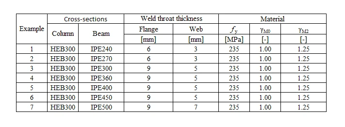
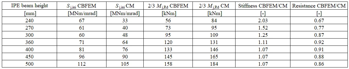
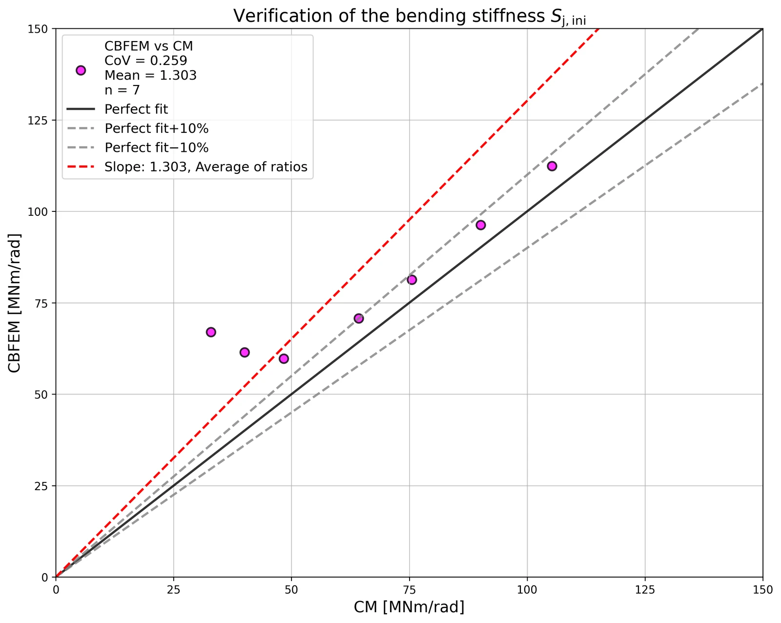
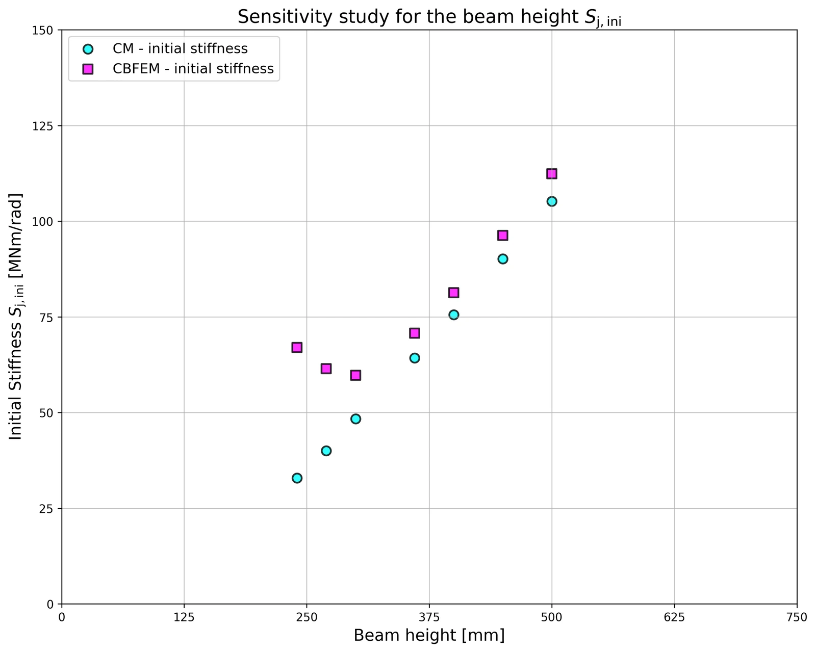
Verification of stiffness
The rotational stiffness calculated by CBFEM is compared with CM. The comparison shows good agreement in initial stiffness and correspondence of joint behavior. The calculated stiffness from CBFEM and CM are summarised in Tab. 10.1.3.
A comparison of the global behavior of a welded eaves moment joint described by a moment-rotation diagram is prepared. The joint is analyzed, and the stiffness of the connected beam is calculated. The main characteristic is the initial stiffness calculated at 2/3Mj,Rd, where Mj,Rd is the design moment resistance of the joint. The moment-rotation diagram is shown in Fig. 10.1.1.
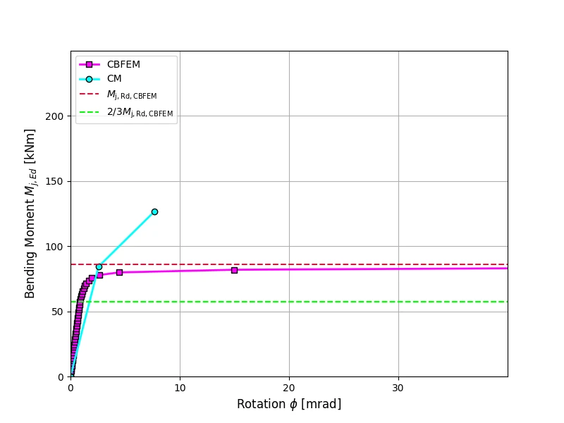
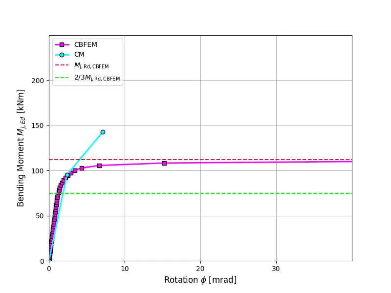
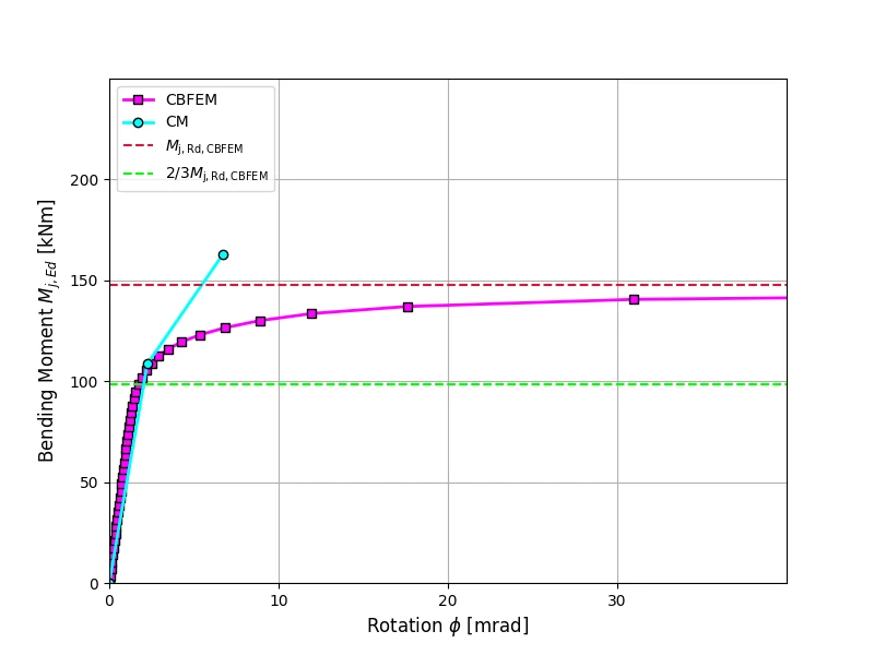
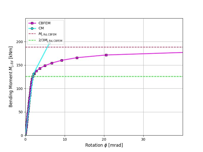
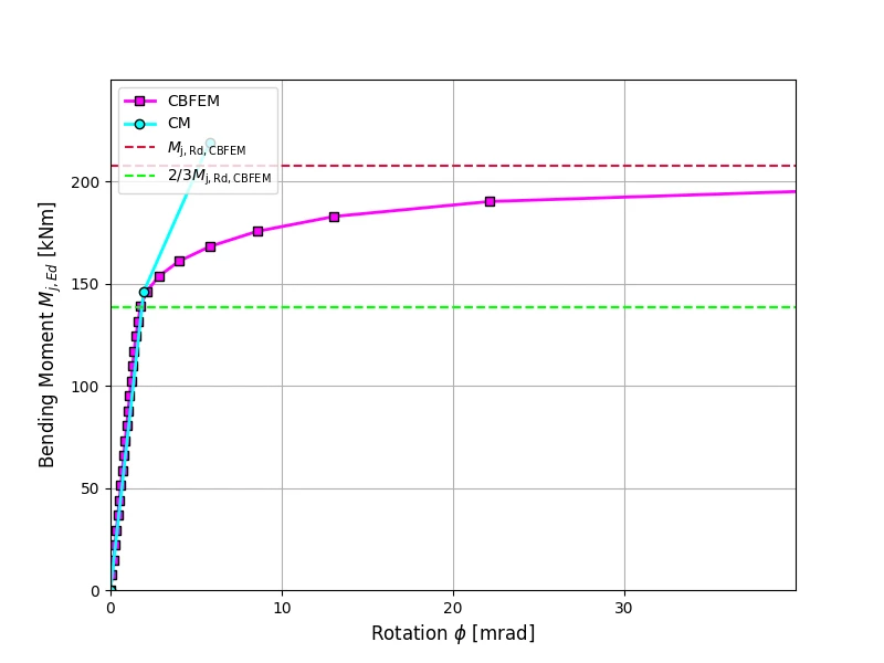
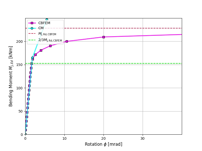
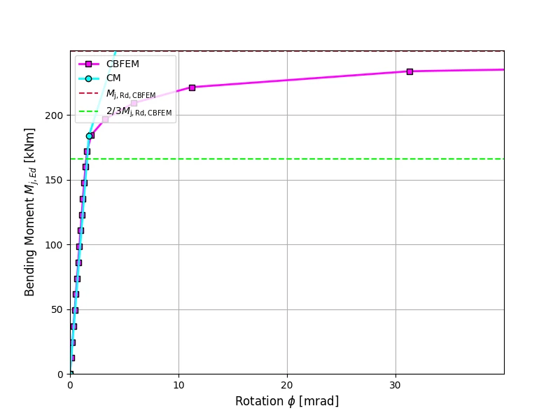
Benchmark case
Inputs
Beam and column
- Steel S235
- Column HEB 300
- Beam IPE 400
- Flange weld throat thickness af = 9 mm
- Web weld throat thickness aw = 5 mm
- Column offset s = 150 mm
- Double fillet weld
Outputs
- Design resistance
- Load
- Secant rotational stiffness
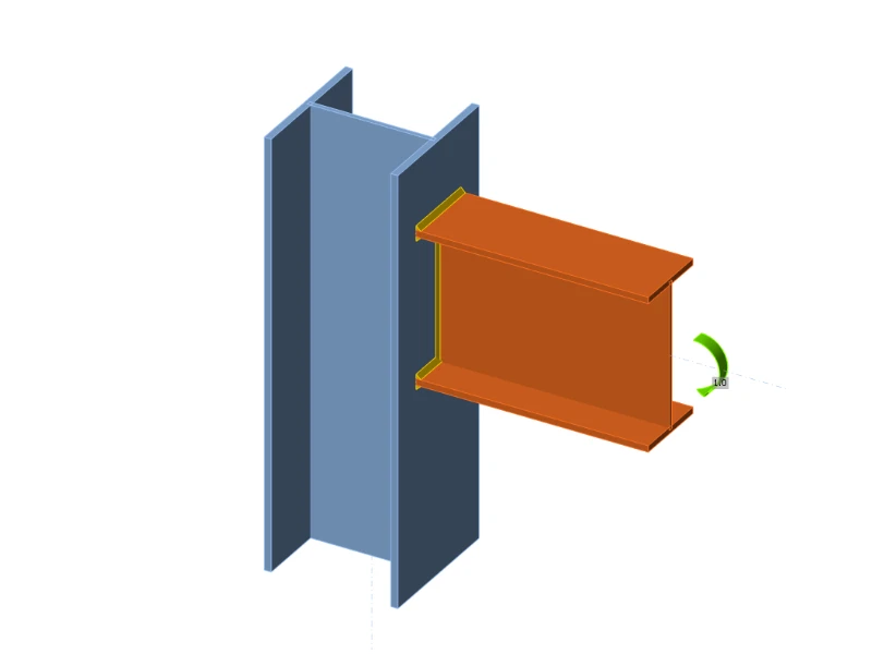
Bending stiffness of bolted joint of open sections
10.2.1 Description
The prediction of rotational stiffness is verified on a bolted eaves moment joint. A bolted joint of open section column HEB and beam IPE is studied and the joint’s behaviour is described on moment-rotation diagram. The results of analytical model by the component-based finite element method (CBFEM) are compared with the component method (CM). The numerical results in form of a benchmark case are available.
10.2.2 Analytical model
The rotational stiffness of a joint should be determined from deformation of its basic components, which are represented by the stiffness coefficient ki. The rotational stiffness of the joint Sj is obtained from:
where
— the stiffness coefficient for the joint component i;
— the lever arm, see 6.2.7;
— the stiffness ratio, see 6.3.1.
The joint components that are taken into account in this example are column web panel in shear k1 which equals infinity for a stiffened column and a single equivalent stiffness coefficient keq for end-plate joint with two or more bolt-rows in tension.
where
— distance from the bolt row to beam bottom flange see Drawing 10.2.1
— the stiffness coefficient for the joint component i
— is the equivalent lever arm

An open section beam IPE 330 is connected with bolted end-plate to a column HEB 200 in the example. The end-plate thickness is 15 mm, the bolt type is M24 8.8 and the assembly is shown in Fig. 10.2.1. Other examples have different column cross-sections. The stiffeners are inside column opposite to beam flanges with thickness of 15 mm. Beam flanges are connected to the end-plate with welds throat thickness of 8 mm. The beam web is connected with weld throat thickness of 5 mm. Plasticity is applied in welds. The material of the beam, column and end-plate is S235. The joint is loaded in bending. The design resistance is limited by the component column web panel in shear. The calculated stiffness coefficients of the basic components, initial stiffness, stiffness by design resistance and rotation of the beam are summarised in Tab. 10.2.1. Joints with column height below 260 mm had the web panel in shear failure mode, other had beam flange in tension, so their bending resistances are equal.
Tab. 10.2.1 Results of the analytical model (Component method)


10.2.3 Verification of stiffness
Detailed information about the prediction of stiffness in CBFEM may be found in chapter 3.9. The CBFEM analyses allows to calculate secant rotational stiffness in any stages of loading. The design resistance is reached by 5% plastic strain in a component column web panel in shear. The rotational stiffness calculated by CBFEM compared with CM. The comparison shows good agreement in initial stiffness and correspondence of joint’s behavior. The calculated stiffness from CBFEM and CM are summarized in Fig 10.2.2.
Tab. 10.2.2 Verification CBFEM to CM


10.2.4 Global behavior and verification
A comparison of the global behavior of a bolted eaves moment joint described by the moment-rotation diagram is prepared. The joint is analyzed and the stiffness of the connected beam is calculated. The main characteristic is the initial stiffness calculated by 2/3 Mj,Rd, where Mj,Rd is the design moment resistance of the joint. Mc,Rd stands for a design moment resistance of the analysed beam. The moment-rotation diagrams are shown in Fig. 10.2.6-10.2.16


10.2.5 Benchmark case
Inputs
Beam and column
- Steel S235
- Column HEB200
- Beam IPE330
Weld
- Flange weld throat thickness af = 8 mm
- Web weld throat thickness aw = 5 mm
End-plate
- Thickness tp = 15 mm
- Height hp = 450 mm
- Width bp = 200 mm
- Bolts M24 8.8
- Bolts assembly in Fig. 10.2.1
Column stiffeners
- Thickness ts = 15 mm
- Width bs = 95 mm
- Related to beam flange, position upper and lower
- Weld throat thickness as = 6 mm
End-plate stiffener
- Thickness tst = 10 mm
- Height hst = 90 mm
- Weld throat thickness ast = 5 mm
Outputs
- Load Mj,Ed = 2/3 Mj,Rd = 70 kNm
- Secant rotational stiffness Sjs = 40 MNm/rad

Prequalified joints for seismic applications
Prequalified joints for seismic applications
12.1 EQUALJOINTS project
The European research project EQUALJOINTS provides prequalification criteria of steel joints for the next version of EN 1998-1. The research activity covered the standardization of design and manufacturing procedures for a set of bolted joint types and a welded reduced beam section with heavy profiles designed to meet different performance levels. There was also the development of a new loading protocol for European prequalification, representative of European seismic demand. The experimental campaign devoted to the cyclic characterization of both European mild carbon steel and high strength bolts achieved the required behavior for four types of pre-qualified joints: haunched bolted joints, unstiffened extended end plate bolted joints, stiffened extended end plate bolted joints, and welded reduced beam section joints; see Fig. 12.1.1. The results experimentally reached within the EQUALJOINJTS project are summarised in (Stratan et al. 2017) and (Tartaglia and D’Aniello, 2017).

Fig. 12.1.1 Structural joints prequalified in EQUALJOINTS project
12.2 End plate joints
The extended stiffened end plate bolted connections are most common among European steel fabricating industries and are widely used in European practice as moment-resistant joints in low and medium-rise steel frames thanks to the simplicity and the economy of fabrication and erection. The design criteria and related requirements for bolted extended stiffened end plate beam-to-column joints are deeply investigated and critically discussed and currently codified in EN 1998-1:2005 based on a parametric study based on finite element analyses. Unfortunately, capacity design procedure was developed only in the framework of component method. It also accounts for the presence of ribs and is able to control the joint response for different performance levels.
Unstiffened extended end plate joints are commonly used in steel construction to connect steel I or H beam to steel I or H column in the case where significant bending moments have to be transferred. This configuration allows an easy erection by bolting while welding the end plate to the beam is automated in shop. The bending resistance of the connection is mostly lower than the bending resistance of the connected members. Therefore, such joints are considered as partial strength. Reaching an equal strength situation, in which the plastic resistance of the joint is roughly equal to the plastic resistance of the beam section, may be achieved through appropriate design. Their ductility in bending depends highly on the detailing of the joints, which influences the failure mode (Jaspart, 1997). If the joint component governing the failure is a ductile one, and if the resistance of the brittle active components is significantly higher, a ductile joint response may be reached. In the opposite case, no reliance should be made on the capacity of the joint to form plastic hinges and redistribute internal forces to absorb energy in a seismic area.
For the welded reduced beam section moment resisting connections, also referred to as dog-bone, two main strategies were adopted by strengthening the connection or weakening the beam. Among these two options for the profile of section reduction, the radius cut tends to exhibit a relatively more ductile behavior, delaying the ultimate fracture (Jones et al. 2002). However, the work showed that reduced beam section members are more prone to lateral-torsional buckling due to the decreased area of their flanges. Further experimental and analytical research focusing on the application of deep columns (Zhang and Ricles, 2006) indicated that the presence of a composite floor slab may greatly reduce the amount of twisting developing in the column, as it offers bracing to the beam and reduces the lateral displacement of the bottom flange.
According to the design procedure developed within the project EQUALJOINTS, the joint comprises three macro-components: the column web panel, the connection zone, and the beam zone; see Fig. 12.2.1. Each macro-component is individually designed according to specific assumptions, and then capacity design criteria are applied in order to obtain three different design objectives defined to assess the joint: full strength, equal strength, and partial strength joints. Full strength joints are designed to guarantee the formation of all plastic deformations into the beam, which is consistent with EN 1998-1:2005 strong column – weak beam capacity design rules. Equal strength joints are theoretically characterized by the contemporary yielding of all macro-components, i.e. connection, web panel, and beam. Partial strength joints are designed to develop the plastic deformation only in the connection or column web panel. According to the resistance of the connection and column web panel macro-components for both equal and partial strength joints, an additional classification can be introduced. For strong web panel, the plastic demand is concentrated in the connection for partial strength joint or in the connection and in the beam for equal strength joint. In balanced web panel, the plastic demand is distributed between the connection and the column web panel for partial strength joint and in the connection, web panel, and the beam for equal strength joint. For weak web panel, the plastic demand is concentrated in the column web panel for partial strength joint or in the web panel and in the beam for equal strength joint.

Fig. 12.2.1 Division of joint into macro components
The joint ductility depends on the type of failure mode and the corresponding plastic deformation capacity of the activated component. Deformation capacity may be roughly predicted by satisfying the developed criteria for CM or more precisely calculated by CBFEM. The examples of design of two prequalified joint configurations described in EQUALJOINJTS project materials and in ANSI/AISC358-16 standard are presented below considering the behavior of macro components separately.
12.2.1 Validation
The CBFEM models of rigidity, load-bearing capacity, and deformation capacity of pre-qualified joints were validated by Montenegro (2017) on a set of experiments available from EQUALJOINT project. The examples of structural solutions are in Fig. 12.2.2. The results of validation of the failure mode are shown in Fig. 12.2.3. The summary of validation of resistance and deformation capacity for 15 % strain are shown in Figs 12.2.4 and 12.2.5.

Fig 12.2.2 Joints used for validation and verification a) EH2- TS-35-M and EH2-TS-45-M, b) ES1-TS-F-M and ES3-TS-F-M, c) E1-TS-E-M and E2-TS-E-M

Fig. 12.2.3 Validation of failure mode of CBFEM on the extended end plate joints with haunch E1-TS-F-C2 (Tartaglia and D’Aniello, 2017)

Fig.12.2.4 Validation of resistance of CBFEM on experiments from EQUALJOINTS project

Fig. 12.2.5 Validation of rotational capacity of CBFEM on experiments from EQUALJOINTS project
12.2.2 Verification
The CBFEM model was verified to CM according to Ch. 6 in EN 1993-1-8:2006. The selection of results is presented in Tab.12.2.1 and Fig 12.2.6. The results show the loss of accuracy of CM for larger joints, where the rough assumption of lever arm is guiding the accuracy.
Tab. 12.2.1 Verification of CBFEM to CM
| Typology | Resistance | |||
| # | CM | CBFEM | CBFEM/CM | Decisive component |
| MR [kNm] | MR [kNm] | [%] | ||
| Haunched joint | ||||
| EH2-TS35-M | 901,2 | 889 | 1 | Endplate in bending |
| EH2-TS45-M | 959,3 | 875 | 10 | Endplate in bending |
| 4.2 | 876,1 | 1 016 | −16 | Column flange in bending |
| 264 | 545,4 | 573 | −5 | Column flange in bending |
| 267 | 1 998,9 | 2 100 | −5 | Endplate in bending |
| Extended stiffened joint | ||||
| ES1-TS-F-M | 547,5 | 533 | 3 | Column flange in bending |
| ES3-TS-F-M | 1389 | 1 920 | −27 | Column flange in bending |
| Extended unstiffened joint | ||||
| E1-TB-E-M | 347,8 | 389 | −11 | Endplate in bending |
| E2-TB-E-M | 577,0 | 681 | −15 | Endplate in bending |

Fig. 12.2.6 Verification of resistance of CBFEM to CM
Three one-sided haunched joints are described in more detail in (Landolfo et al. 2017) and (Equaljoints application). The joints are loaded by both sagging and hogging bending moments and corresponding shear load. The column webs are reinforced by doublers, so the decisive components are T-stubs of either end plate or column flange. The axes of rotation are assumed at the center of the upper beam flange for sagging bending moment and in the middle of the haunch for hogging bending moment. The position of plastic hinge is assumed at the face of the stiffening plate at the end of the haunch. The bending moment at the column face used for check of the connection is increased by the corresponding shear load; see Fig. 12.2.7.

Fig. 12.2.7 Position of plastic hinge, course of bending moment in the haunched joint
Tab. 12.2.2 Resistance of components by CM for haunched joints
| Resistance of components by CM | #4.2 (IPE450 to HEB340) | #264 (IPE360 to HEB280) | #267 (IPE600 to HEB500) |
| Moment at plastic hinge [kNm] | 906 | 543 | 1869 |
| Shear load [kN] | 295 | 148 | 561 |
| Moment at column face [kNm] | 981 | 573 | 2105 |
| Haunch resistance [kNm] | 956 | 582 | 1903 |
| Shear acting on column web [kN] | 1581 | 1035 | 2447 |
| Column web in shear resistance [kN] | 1632 | 1203 | 2774 |
| T-stub - end plate - hogging moment [kNm] | 1019 | 573 | 1999 |
| T-stub - end plate - sagging moment [kNm] | 1081 | 697 | 2318 |
| T-stub - column flange - hogging moment [kNm] | 876 | 545 | 2015 |
| T-stub - column flange - sagging moment [kNm] | 929 | 580 | 2107 |
The strain-hardening factor was chosen 1,2 as suggested by EN 1993-1-8:2006 and Equaljoints project final report (EN 1998-1:2005 suggests value 1,1). Overstrength factor was assumed 1,25 (Landolfo et al. 2017). All steel was grade S355. The resistances of individual components are summarized in Tab. 12.2.2. The checks in bold are failing. Note that haunch resistance is the plastic resistance of the beam section with the haunch at end plate. The strength of the beam is assumed increased by overstrength factor at the location of plastic hinge but not at the end plate. If the overstrength factor was used at the end plate as well, this resistance would be higher. Therefore, the next lowest resistance, the T-stub – end plate, was assumed to govern the joint resistance of joint No. 267. None of the investigated joints meets the requirement for full-strength joint. However, the resistance is very close, and the joints are equal-strength. The column web panel is in all cases strong.
The governing failure mode by CBFEM is failure of bolts with yielding of plates, mainly end plate, column flange, and haunch. According to CBFEM, joints No. 4.2 and No. 264 are full-strength and joint No. 267 equal-strength. Column web panels are strong in all cases.


Fig. 12.2.8 The strains at resistance for a) the whole joint, b) the macro-component bolted end-plate connection only c) the macro-component column web panel in shear with web doublers only, d) the macro-component beam only
12.2.3 Unstiffened extended end-plate joints
For sensitivity study, a prequalified unstiffened extended end-plate joint was selected. The beam IPE 450 is connected to column HEB 300 by an extended end plate 25 mm thick with twelve M30 10.9 bolts, with and without web doubler 10 mm thick. Steel grade S 355 was used for all plates. To determine the contribution of each macro component separately, the material diagram of the selected macro component was elastoplastic, while the rest of the joint was with only elastic material diagram. The strains at the resistance of the whole joint, the column web panel in shear with web doublers only, and the bolted end-plate connection only are compared to the beam macro-component only in Fig. 12.2.8. The influence of each macro-component on the behavior of the joint is presented in Fig. 12.2.9, where column web panel with and without web doublers is shown. The joint behavior shows higher resistance of the connection macro-component.

Fig. 12.2.9 Influence of macro-components, the column web panel with doublers in shear,
the bolted end-plate connection and beam to the behavior of the whole joint
12.2.4 Location of compression center
For end-plate joints, EN 1993-1-8:2006 specifies that the compression center is located in the middle of the thickness of beam flange, or at the tip of the haunch in case of haunched joints. Experimental and numerical results showed that the location of compression center depends on both the joint type and the rotation demand due to the formation of plastic modes with different engagement of each joint component (Landolfo et al. 2017). According to the proposed CM design procedure and based on both experimental and numerical results, contact at about the centroid of the section made by the beam flange and the rib stiffeners is expected, for the stiffened endplate joints or at about 0,5 the haunch height in case of haunched joints. This rough assumption is précised by CBFEM procedure, which gives correct values during loading and initial yielding of parts of a joint.
The presented results show the good accuracy of CBFEM verified to ROFEM validated to EQUALIJOINTS experiments and CM. It brings the possibility to consider the behavior of macro-components separately and the position of neutral axes accurately according to the loading/plastification.
12.3 Welded reduced beam section joint
A prequalified welded reduced beam section joint according to ANSI/AISC 358-16 was selected for this study. The beam IPE 450 is connected to column HEB 300 by butt welds at flanges and fin plate 12 mm thick with three preloaded M30 10.9 bolts, with and without web doubler 10 mm thick; see Fig. 12.3.1. All used steel is grade S355.
The strains at the ultimate resistance of the whole joint and macro component column web panel in shear with web doublers only are shown in Fig. 12.3.2. The influence of each macro-component to the behavior of the joint is presented in Fig. 12.3.3, where column web panel with and without web doublers is shown. The joint shows that the resistances of the joint macro-components are well-optimized.

Fig. 12.3.1 Reduced beam section joint, a) beam with reduced section, b) the column web panel with doublers in shear, the bolted end plate connection,

Fig. 12.3.2 The strains at resistance for a) the whole joint and b) the macro component column web panel with doublers in shear only

Fig. 12.3.3 Influence of macro-components on the behavior of the whole joint on M-φ diagram
References
EN 1993-1-8, Eurocode 3, Design of steel structures – Part 1-8: Design of joints, CEN, Brussels, 2005.
Jones S.L., Fry GT., Engelhardt M.D. Experimental evaluation of cyclically loaded reduced beam section moment connections. Journal of Structural Engineering. 128 (4), 441–451, 2002.
Landolfo R. et al. Design of Steel Structures for Buildings in Seismic Areas, ECCS Eurocode Design Manual. Wiley, 2017.
Stratan A., Maris C, Dubina D, and Neagu C. Experimental prequalification of bolted extended end plate beam to column connections with haunches. ce/papers, 1(2–3), 414–423, 2017.
Tartaglia R, D’Aniello M. Nonlinear performance of extended stiffened end-plate bolted beam-to-column joints subjected to column removal. The Open Civil Engineering Journal Vol 11, Issue Suppl-1, 369–383, 2017.
Zhang X., Ricles J.M. Experimental evaluation of reduced beam section connections to deep columns. Journal of Structural Engineering. 132 (3), 346-357, 2006.